
Research Article Volume 12 Issue 3
Weighted Adya distribution with properties and application
Rama Shanker,1  Kamlesh Kumar Shukla2
1Department of Statistics, Assam University, Silchar, Assam, India
2Department of Community Medicine, Noida International Institute of Medical Science, India
Correspondence: Kamlesh Kumar Shukla, Department of Community Medicine, Noida International Institute of Medical Science, India
Received: May 15, 2023 | Published: May 31, 2023
Citation: Shanker R, Shukla KK. Weighted Adya distribution with properties and application. Biom Biostat Int J. 2023;12(3):68-74. DOI: 10.15406/bbij.2023.12.00386
Download PDF
Abstract
In this paper a weighted version of Adya distribution which includes Adya distribution has been suggested for modeling lifetime data. The natures of descriptive statistics including coefficients of variation, skewness, kurtosis, and index of dispersion have been studied. The reliability measures including hazard rate function, reversed hazard rate function, mean residual life function and stochastic ordering have been studied. Method of maximum likelihood estimation has been discussed for estimating the parameters. A simulation study has been presented to know the performance of maximum likelihood estimates of parameters. The goodness of fit of the proposed distribution has been explained with a real lifetime data.
Keywords: Adya distribution, moments, reliability properties, maximum likelihood estimation, application
Introduction
As we know that the basic purpose of distribution theory is to determine a reasonable distributional model for the data arising from different fields of knowledge. And once the distributional model of the data is determined, characterization of distribution, computation of confidence intervals of parameters and critical regions for hypothesis tests can easily be done. It has been observed that the discrete or continuous data that we are getting are stochastic in nature and the existing distributions are not able to explain the true nature of data and this is the reasons for the search for new distributions. Further, it has been observed that many times the true nature of data can be better explained by weighted distribution with appropriate weight function. The concept of weighted distributions was firstly introduced by Fisher1 to model ascertainment biases which were later reformulated by Rao2 in a unifying theory for problems where the observations fall in the category of non-experimental, non-replicated and non-random. When observations are recorded by an investigator in the nature according to some stochastic model, the distribution of the recorded observations will not have the original distribution unless every observation is given an equal chance of being recorded. For instance, let the original observation
comes from a distribution having probability density function (pdf)
, where
may be a parameter vector and the observation
is recorded according to a probability re-weighted by weight function
,
being a new parameter vector, then
comes from a distribution having pdf
(1.1)
Note that such types of distribution are known as weighted distributions. The weighted distributions with weight function
are called length biased distributions or simple size-biased distributions. Patil et al.3,4 have examined some general probability models leading to weighted probability distributions and their applications and showed the occurrence of
in a natural way in problems relating to sampling.
The study of weighted distributions is useful in distribution theory because it provides a new understanding of the existing standard probability distributions and it provides methods for extending existing standard probability distributions for modeling lifetime data due to introduction of additional parameter in the model which creates flexibility in their behavior. Weighted distributions occur in modeling datasets having clustered sampling, heterogeneity, and extraneous variation.
Shanker et al.5 introduced a one parameter lifetime distribution named Adya distribution (AD) having pdf and cdf
(1.2)
(1.3)
Obviously Adya distribution is a convex combination of an exponential
distribution, a gamma
distribution and a gamma
distribution with their mixing proportions
,
and
, respectively.
Shanker et al.5 discussed its statistical properties including coefficient of variation, skewness, kurtosis, index of dispersion, hazard rate function, mean residual life function, stochastic ordering, mean deviations from the mean and the median, Bonferroni and Lorenz curves, stress-strength reliability along with estimation of parameter using maximum likelihood estimation and applications to model lifetime data from engineering and biomedical sciences.
The main purpose of the present paper is to derive weighted version of Adya distribution and discuss its important statistical properties. Its statistical properties including behaviour of pdf, cdf, hazard rate function, mean residual life function and moments based descriptive measures. Maximum likelihood estimation has been discussed to estimate parameters of the distribution. The simulation study to know the performance of maximum likelihood estimates is presented. Finally, an application of the proposed weighted Adya distribution has been presented to test its goodness of fit with other distributions.
Weighted Adya distribution
Considering the weight function
in (1.1) and using the pdf of Adya distribution from (1.2), the pdf of weighted Adya distribution (WAD) can be expressed as
, (2.1)
where
is the complete gamma function defined as
(2.2)
It can be easily shown that Adya distribution is a particular case of WAD at
. Like Adya distribution, the pdf of Weighted Adya distribution can be easily expressed as a convex combination of gamma
, gamma
and gamma
distributions. We have
, (2.3)
where
,
,
and
.
The survival (reliability) function of WAD can be obtained as
, (2.5)
where
the upper incomplete gamma function defined as
(2.6)
Thus, the cdf of WAD can thus be given by
Graphs of the pdf and the cdf of WAD for varying values of the parameters
are shown in Figures 1 & 2 respectively.
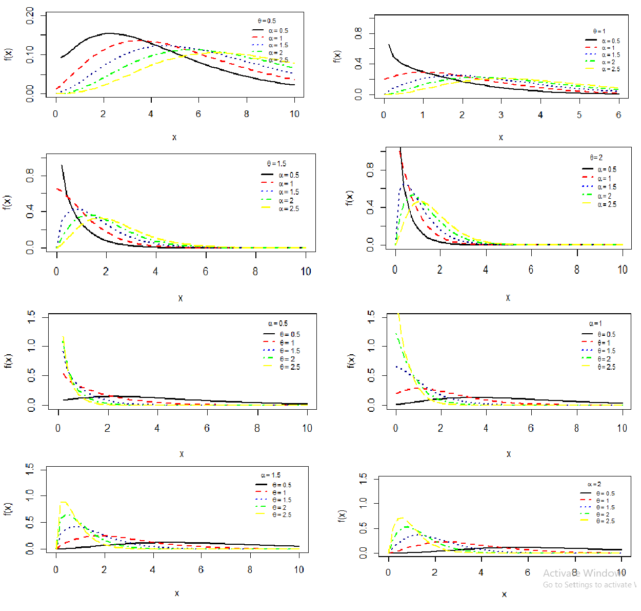
Figure 1 pdf of WAD for varying values of
.
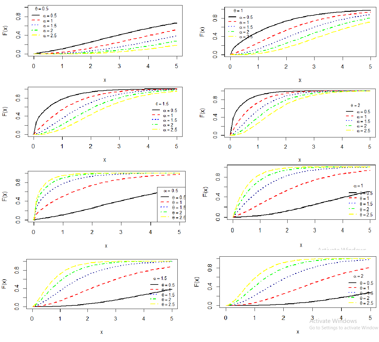
Figure 2 cdf of WAD for varying values of
.
Moments based measures
The
th moment about origin
of WAD can be obtained as
(3.1)
The first four moments about origin of WAD thus can be obtained as
.
Using the relationship between central moments and moments about origin, the central moments of WAD can be obtained as
Thus the coefficient of variation (C.V), coefficient of skewness
, coefficient of kurtosis
, and index of dispersion
of WAD are obtained as
.
It should be noted that these moments of WAD reduce to the corresponding moments of Adya distribution at
. Behaviors of coefficient of variation (C.V), coefficient of Skewness (S.K), coefficient of kurtosis (S.K.) and index of dispersion (I.D) of WAD are drawn for varying values of parameters and are shown in Figures 3–6 respectively.
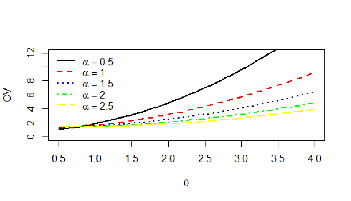
Figure 3Graphs of C.V of WAD for varying values of parameters
.
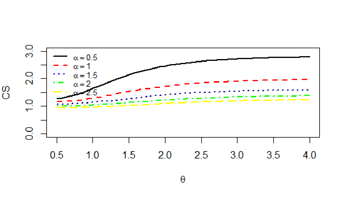
Figure 4 Graphs of C.S of WAD for varying values of parameters
.
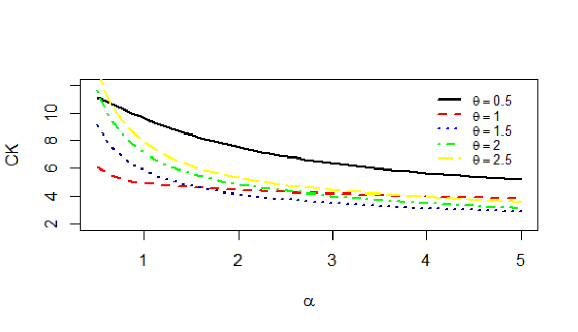
Figure 5 Graphs of C.K of WAD for varying values of parameters
.
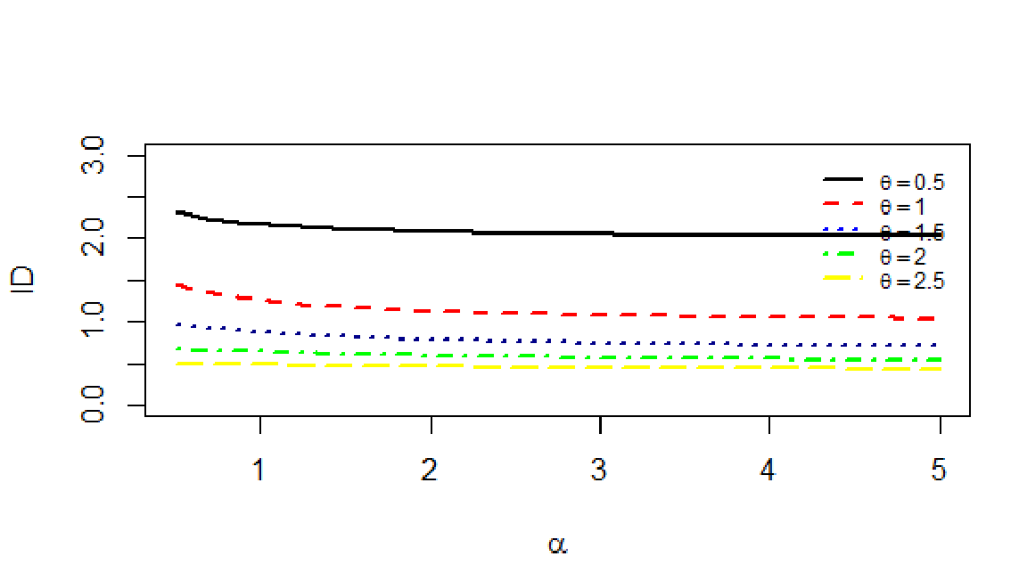
Figure 6 Graphs of I.D of WAD for varying values of parameters
.
Moment generating function
The moment generating function of WAD can be obtained as
.
.
It can be easily verified that the coefficient of
in
gives the same
as given by (3.1).
Harmonic mean
The harmonic mean of WAD can be obtained as
.
Reliability measures
There are some important reliability measures of a distribution namely, the hazard rate function, reverse hazard rate function, Mills ratio and inverse Mills ratio, the mean residual life function and Stochastic ordering. In this section these reliability measures for WAD have been discussed.
Hazard rate function
The hazard (or instantaneous failure rate function) plays a crucial role in reliability and survival analysis, as it defines the conditional probability of failure of an item in the next very small units of time
, given that it did not fail before
. Suppose
is a random variable with cdf
. If
is absolutely continuous, then the random variable
has a probability density function
. The hazard rate (HR) function
of
is defined as
The hazard (or failure rate) function,
of WAD can be obtained as
.
Graphs of
of WAD for varying values of parameters
are shown in Figure 7. It is obvious that for varying values of parameters, the shapes of hazard rate function of WAD are changing and it can be used for data of various nature.
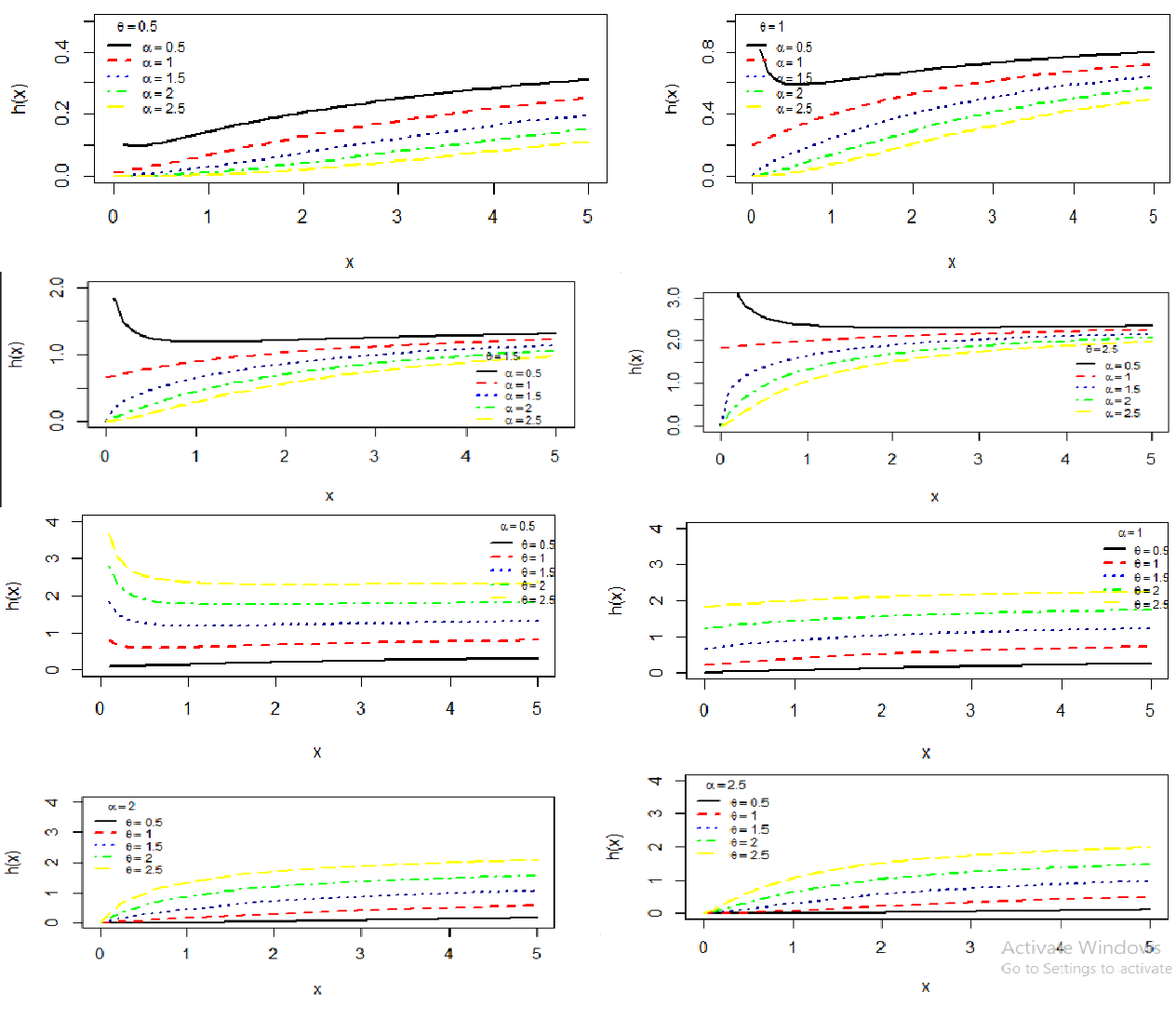
Figure 7
of WAD for varying values of parameters
.
Reverse hazard rate function
A function closely related to the hazard rate function is the reverse hazard rate function which was firstly introduced by Barlow et al. It is the dual of the hazard rate function and is defined as
.
Thus, the corresponding reverse hazard rate function of WAD can be obtained as
.
Mills ratio and inverse mills ratio
The Mills ratio is defined as the ratio of the complementary cdf to the pdf of a random variable
and is denoted as
and defined as
.
It is also related to the hazard rate function as
The inverse Mills ratio is the ratio of the pdf to the complementary cdf of a random variable
.
Mean residual life function
The mean residual life function
of WAD can be obtained as
It can be easily shown that
.
Graphs of
of WAD for varying values of parameters
are shown in Figure 8.
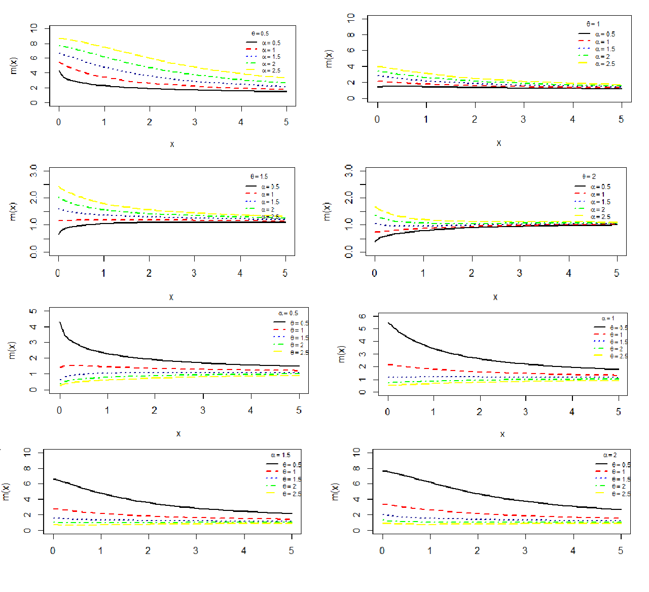
Figure 8
of WAD for varying values of parameters
.
Stochastic ordering
The stochastic ordering of positive continuous random variables is an important tool for judging their comparative behavior. A random variable
is said to be smaller than a random variable
in the
- stochastic order
if
for all
- hazard rate order
if
for all
- mean residual life order
if
for all
- Likelihood ratio order
if
decreases in
.
The following interrelationships due to Shaked & Shanthikumar6 are well known for establishing stochastic ordering of distributions
It can be easily shown that WAD is ordered with respect to the strongest ‘likelihood ratio’ ordering. The stochastic ordering of WAD has been explained in the following theorem:
Theorem: Suppose
WAD
and
WAD
. If
(or
;
), then
and hence
,
and
.
Proof: We have
Now, taking logarithm both sides, we get
This gives
.
Thus for
(or
and
),
. This means that
and hence
,
and
.
Maximum likelihood estimation
Suppose
be a random sample of size
from WAD. The log-likelihood function,
of WAD can be obtained as
The maximum likelihood estimates (MLE’s)
of the parameters
of WAD are the solutions of the following log likelihood equations
where
is the digamma function.
Since these two log likelihood equations cannot be expressed in closed forms, they cannot be solved analytically. However, these two log likelihood equations can be solved using R-software.
A simulation study
In this section, a simulation study has been carried to check the performance of maximum likelihood estimates by taking sample sizes (n=20, 40, 60, 80) for values of
and
&
. Acceptance and rejection method is used to generate random number for data simulation using R-software. The process was repeated 1,000 times for the calculation of Average Bias error (ABE) and MSE (Mean square error) of parameters
and
and are presented in Tables1 & 2 respectively. For the WAD decreasing trend has been observed in ABE and MSE as the sample size increases and this shows that the performance of maximum likelihood estimators is quite good and consistent.
|
n
|
|
ABE(
)
|
MSE (
)
|
ABE (
)
|
MSE (
)
|
|
20
|
0.5
|
-0.0037
|
0.0003
|
-0.0560
|
0.0007
|
|
20
|
1.0
|
-0.0287
|
0.01649
|
-0.0310
|
0.0193
|
|
20
|
1.5
|
-0.0537
|
0.0577
|
-0.0560
|
0.0628
|
|
20
|
2.0
|
-0.0787
|
0.1239
|
-0.0810
|
0.1313
|
|
40
|
0.5
|
0.0022
|
0.0002
|
-0.0225
|
0.0003
|
|
40
|
1.0
|
-0.0103
|
0.0042
|
-0.0099
|
0.0039
|
|
40
|
1.5
|
-0.0227
|
0.0207
|
-0.02249
|
0.0202
|
|
40
|
2.0
|
-0.0353
|
0.0497
|
-0.0349
|
0.0489
|
|
60
|
0.5
|
0.001
|
0.0006
|
-0.0142
|
0.0003
|
|
60
|
1.0
|
-0.0073
|
0.0032
|
-0.0059
|
0.0021
|
|
60
|
1.5
|
-0.0156
|
0.0147
|
-0.0142
|
0.0121
|
|
60
|
2.0
|
-0.0239
|
0.0345
|
-0.0225
|
0.0305
|
|
80
|
0.5
|
0.0001
|
0.0000
|
-0.0117
|
0.0004
|
|
80
|
1.0
|
-0.0061
|
0.0030
|
-0.0055
|
0.0024
|
|
80
|
1.5
|
-0.0124
|
0.0123
|
-0.0117
|
0.0111
|
|
80
|
2.0
|
-0.0186
|
0.0277
|
-0.0180
|
0.0360
|
Table 1 ABE and MSE of parameters at fixed value
|
n
|
|
ABE(
)
|
MSE (
)
|
ABE (
)
|
MSE (
)
|
|
20
|
0.5
|
0.0298
|
0.0177
|
0.0052
|
0.0608
|
|
20
|
1.0
|
0.0048
|
0.0005
|
0.0302
|
0.0182
|
|
20
|
1.5
|
-0.0202
|
0.0081
|
0.0052
|
0.0005
|
|
20
|
2.0
|
-0.0452
|
0.0408
|
-0.0198
|
0.0078
|
|
40
|
0.5
|
0.0166
|
0.0112
|
0.0162
|
0.0678
|
|
40
|
1.0
|
0.0041
|
0.0007
|
0.0287
|
0.0329
|
|
40
|
1.5
|
-0.0084
|
0.0028
|
0.0162
|
0.0104
|
|
40
|
2.0
|
-0.0208
|
0.0174
|
0.0036
|
0.0005
|
|
60
|
0.5
|
0.0084
|
0.0094
|
0.0067
|
0.0329
|
|
60
|
1.0
|
0.0001
|
0.0000
|
0.0151
|
0.0136
|
|
60
|
1.5
|
-0.0082
|
0.0040
|
0.0067
|
0.0027
|
|
60
|
2.0
|
-0.0165
|
0.0164
|
-0.0015
|
0.0001
|
|
80
|
0.5
|
0.0070
|
0.0039
|
0.0066
|
0.0293
|
|
80
|
1.0
|
0.0007
|
0.0004
|
0.0129
|
0.0133
|
|
80
|
1.5
|
-0.0055
|
0.0024
|
0.0066
|
0.0035
|
|
80
|
2.0
|
-0.0117
|
0.0109
|
0.0004
|
0.0001
|
Table 2 ABE and MSE of parameters at fixed value
A numerical example
In this section application and the goodness of fit of WAD has been discussed with the following real lifetime data relating to the lifetime of a certain device reported by Sylwia7 and the observations are 0.0094, 0.0500, 0.4064, 4.6307, 5.1741, 5.8808, 6.3348, 7.1645, 7.2316, 8.2604, 9.2662, 9.3812, 9.5223, 9.8783, 9.9346, 10.0192, 10.4077, 10.4791, 11.0760, 11.3250, 11.5284, 11.9226, 12.0294, 12.0740, 12.1835, 12.3549, 12.5381, 12.8049, 13.4615, 13.8530.
For this data set, WAD has been fitted along with one parameter exponential and Adya distributions and two-parameter distributions including weighted Lindley distribution (WLD) introduced by Ghitany et al.,8 quasi Lindley distribution (QLD) of Shanker & Mishra,9 a two-parameter Lindley distribution (TPLD-I) of Shanker & Mishra,10 a two-parameter Lindley distribution (TPLD-II) of Shanker et al.11 and Weibull distribution introduced by Weibull.12 The pdf and cdf of the considered distributions: WLD, Weibull, TPLD-I, TPLD-II, QLD and exponential distribution are given in Table 3. The ML estimates, values of
, Akaike Information criteria (AIC), K-S statistics and p-value of the fitted distributions are presented in Table 4. The AIC and K-S Statistics are computed using the following formulae:
and
, where
= the number of parameters,
= the sample size ,
is the empirical (sample) cumulative distribution function, and
is the theoretical cumulative distribution function. The best distribution is the distribution corresponding to lower values of
, AIC, and K-S statistics.
|
Distributions
|
Pdf
|
Cdf
|
|
WLD
|
|
|
|
Weibull
|
|
|
|
TPLD-I
|
|
|
|
TPLD-II
|
|
|
|
QLD
|
|
|
|
Exponential (ED)
|
|
|
Table 3 The pdf and the cdf of fitted distributions
|
Distribution
|
ML Estimates
|
|
AIC
|
K-S
|
P-value
|
|
θ
|
α |
|
WAD
|
0.2303
|
0.132
|
179.31
|
183.31
|
0.276
|
0.010
|
|
WLD
|
0.1733
|
0.7537
|
183
|
187
|
0.281
|
0.012
|
|
Weibull
|
0.0258
|
1.6168
|
185.45
|
189.45
|
0.278
|
0.014
|
|
TPLD-I
|
0.2001
|
1.1774
|
183.74
|
187.74
|
0.275
|
0.016
|
|
TPLD-II
|
0.2002
|
0.849
|
183.74
|
187.74
|
0.275
|
0.016
|
|
QLD
|
0.2001
|
0.2356
|
183.74
|
187.74
|
0.275
|
0.016
|
|
AD
|
0.3314
|
-------
|
187.43
|
189.43
|
0.338
|
0.001
|
|
Exponential
|
0.1106
|
--------
|
192.09
|
194.09
|
0.314
|
0.004
|
Table 4 MLE’s, - 2ln L, AIC, K-S statistics and p-values of the fitted distributions
The variance-covariance matrix and the 95% confidence intervals (CI’s) of the ML estimates of the parameters
and
of WAD are presented in Table 5. From the goodness of fit in Table 4 and the fitted plots of the distribution for the considered datasets in Figure 9 shows that WAD gives much closure fit as compared to other considered distributions.
|
Parameters
|
Variance-covariance matrix
|
95 % CI
|
| |
|
Lower Upper
|
|
|
0.001109402 0.00279572
|
0.17450148 0.3121785
|
|
|
0.002795720 0.01862830
|
0.01988068 0.6389076
|
Table 5 Variance-Covariance matrix and 95% confidence intervals (CI’s) of the ME estimates
of parameters
for the given dataset
The profile of likelihood estimates of parameters
of WAD for the given dataset is shown in Figure 9. Also, the fitted plots of the considered dataset for WAD are shown in Figure 10.
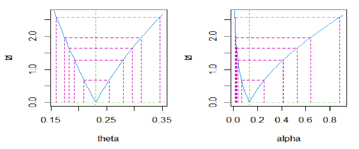
Figure 9 Profile of the likelihood estimates
of WAD for the given dataset.

Figure 10 Fitted plots of the two-parameter distributions for the given dataset.
Concluding remarks
In this paper a two-parameter weighted Adya distribution (WAD) which includes one parameter Adya distribution as special case has been suggested for modeling lifetime data. Some of its properties including shapes of probability density function, moments-based measures including coefficients of variation, skewness, kurtosis, and index of dispersion; hazard rate function, mean residual life function and stochastic ordering have been studied. Method of maximum likelihood estimation has been discussed for estimating the parameters. The simulation study has been presented to know the performance of parameters. The goodness of the proposed distribution has been explained with a real lifetime data and the fit has been found to be quite satisfactory over one parameter and two parameter lifetime distributions.
Acknowledgments
Conflicts of interest
The authors declare that there are no conflicts of interest.
Funding
References
- Fisher RA. The effects of methods of ascertainment upon the estimation of frequencies. Ann Eugenics. 1934;6:13–25.
- Rao CR. On discrete distributions arising out of methods of ascertainment. Patil GP, editor. Classical and contagious discrete distributions. Calcutta: Statistical Publishing Society; 1965:320–332.
- Patil GP, Rao CR. The weighted distributions: A survey and their applications. Krishnaiah PR, editor. In applications of Statistics: Amsterdam: North Holland Publications Co; 1977.
- Patil GP, Rao CR. Weighted distributions and size-biased sampling with applications to wild-life populations and human families. Biometrics. 1978;34:179–189.
- Shanker R, Shukla KK, Ranjan A, et al. Adya distribution with properties and application. Biom Biostat Int J. 2021;10(3):81–88.
- Shaked M, Shanthikumar JG. Stochastic orders and their applications. New York: Academic Press; 1994.
- Sylwia KB. Makeham's generalized distribution. Computational Methods in Science and Technology. 2007;13(2):113–120.
- Ghitany ME, Alqallaf F, Al Mutairi DK, et al. A two-parameter weighted Lindley distribution and its applications to survival data. Mathematics and Computers in simulation. 2011;81(6):1190–1201.
- Shanker R Mishra A. A Quasi Lindley distribution. African Journal of Mathematics and Computer Science Research. 2013(a);6(4):64–71.
- Shanker R, Mishra A. A two-parameter Lindley distribution. Statistics in Transition new Series. 2013b;14(1):45–56.
- Shanker R, Sharma S, Shanker R. A two parameter Lindley distribution for modeling waiting and survival times data. Applied Mathematics. 2013;4(2):363–368.
- Weibull W. A statistical distribution of wide applicability. Journal of Applied Mathematics. 1951;18:293–297.

©2023 Shanker, et al. This is an open access article distributed under the terms of the,
which
permits unrestricted use, distribution, and build upon your work non-commercially.


