In this paper, we introduced a four-parameter probability model called Weibull-Inverse Lomax distribution with decreasing, increasing and bathtub hazard rate function. The WIL distribution density function is J-shaped, positively skewed, and J-shaped in reverse. Some of the mentioned distribution’s statistical characteristics are provided including moments, order statistics, entropy, mean, variance, moment generating function, and quantile function. The method of maximum likelihood estimation was used to estimate the parameters of the model.  The distribution’s importance is proved by its implementation to the bladder cancer data set. Goodness-of-fit of this distribution by various techniques demonstrates that the WIL distribution is empirically better for lifetime application.

Keywords: entropy, moments, moment generating functions, Weibull-Inverse lomax distribution

Real life datasets can be fitted by utilizing a lot of existing statistical distributions. However, most of these real-world datasets does not follow these existing statistical distributions. Hence, the need to propose/develop new distributions that could describes some of these situations better and can also provide a better flexibility in the modelling of real-world data sets compared with the baseline distributions. As a result of this fact, researchers have developed many statistical families of distributions and study most of their properties. These include: The Transmuted Weibull lomax distribution by Afify et al.,¹ kumaraswamy Marshal-olkin family by Afify et al.,² Lomax generator by Cordeiro et al.,³ the weibull exponential by Oguntunde et al.,⁴ kumaraswamy-pareto by Bourguignon et al.,⁵ weibull-G family by Bourguignon et al.,⁶ the weibull-dagum distribution by Tahir et al.,⁷ the generalized transmuted-G family of distributions by Nofal et al.,⁸ among others. Recently, a lot of extensions of distributions have been proposed and studied based on the Weibull-G family of distributions by Bourguignon et al.,⁶ Among them is the Tahir, Merovci, Afify, Yousof, and  Oguntunde et al.^9-12,4 to mention but few.

Inverse Lomax distribution is a member of Beta-type distribution. Other members of the family include Dagum, lomax, Fisk or log-Logistics, Singh maddala, generalized beta distributions of the second kind among others, as in Kleiber et al.¹³ If a random variable say Z has a Lomax distribution, then has an Inverse Lomax distribution (ILD). It has been utilized to get the Lorenz ordering relationship among ordered statistics;.¹⁴ Apart from this, it has also many applications in economics, actuarial sciences, and stochastic modeling Kleiber C, Kotz S & Kleiber C^13,14  have applied this model on geophysical data, specifically on the sizes of land fires in California state of US. Rahman et al.¹⁵  have discussed the estimation and prediction challenges for the inverse Lomax distribution via Bayesian approach. Yadav et al.¹⁶ have used this distribution for reliability estimation based on Type II censored observations. Some details about the Inverse Lomax distribution including its applications are available in Reyad and Othman, Falgore et al., Maxwell et al., and Hassan and Mohamed.^17-23

The main aim of this paper is to provide an extension of the Inverse-Lomax distribution using the Weibull-G generator by Bourguignon et al.⁶ Therefore, we propose the Weibull-Inverse lomax (WIL) distribution by adding two extra shape parameters to the Inverse Lomax distribution.

The Inverse-Lomax distribution and Weibull G family

The probability density function (pdf) and cumulative distribution function (cdf) of ILD are given by the following equations as define by Yadav et al.¹⁶ as:

$g(x;\gamma \mathrm{,}\lambda )=\frac{\gamma \lambda }{x^2}{(1+\frac{\gamma }{x})}^{-(1+\lambda )}$ (1)

$G\mathrm{<mo\; stretchy="false">(</mo>}x\mathrm{<mo>;</mo>}\gamma \mathrm{,}\lambda \mathrm{<mo\; stretchy="false">)</mo><mo>=</mo>}{\left(1+\frac{\gamma }{x}\right)}^{-\lambda }$ (2)

where x > 0, γ, λ > 0 are scale and shape parameters respectively.

$Letg\left(x;\eta \right)andG\left(x;\eta \right)$ denote the probability density function (pdf) and cumulative distribution function (cdf) of a baseline with parameter vector η and also consider the Weibull Cumulative Density Function (cdf) $F\left(x\right)=1-exp\left(-d{x}^p\right)\left(for x>0\right)$ with positive parameters d and p. Based on this cdf, Bourguignon et al.⁶  replaced the argument x by $G\left(x;\eta \right)/1-G\left(x;\eta \right)$ , and defined the cdf and the pdf of the Weibull-G family by:

$F(x;\alpha \mathrm{,}\beta \mathrm{,}\eta )=1-\exp \{-\alpha {\left[\frac{G(x;\eta )}{\overline{G(}x;\eta )}\right]}^{\beta }\}\mathrm{,}x\in \Im \subseteq \Re ;\alpha \mathrm{,}\beta >0,$ (3)

where G(x;η) is any baseline cdf which depends on a parameter vector η.

$f\mathrm{<mo\; stretchy="false">(</mo>}x\mathrm{<mo>;</mo>}\alpha \mathrm{,}\beta \mathrm{,}\eta \mathrm{<mo\; stretchy="false">)</mo><mo>=</mo>}\alpha \beta g\mathrm{<mo\; stretchy="false">(</mo>}x\mathrm{<mo>;</mo>}\eta \mathrm{<mo\; stretchy="false">)</mo>}\frac{G{\mathrm{<mo\; stretchy="false">(</mo>}x\mathrm{<mo>;</mo>}\eta \mathrm{<mo\; stretchy="false">)</mo>}}^{\beta -1}}{\overline{G}{\mathrm{<mo\; stretchy="false">(</mo>}x\mathrm{<mo>;</mo>}\eta \mathrm{<mo\; stretchy="false">)</mo>}}^{\beta +1}}\exp \left\{-\alpha {\left[\frac{G\mathrm{<mo\; stretchy="false">(</mo>}x\mathrm{<mo>;</mo>}\eta \mathrm{<mo\; stretchy="false">)</mo>}}{\overline{G}\mathrm{<mo\; stretchy="false">(</mo>}x\mathrm{<mo>;</mo>}\eta \mathrm{<mo\; stretchy="false">)</mo>}}\right]}^{\beta }\right\}$ (4)

The interpretation of the family of distribution above as in Cooray²¹ is as follows. Let L be a lifetime random variable having a continuous cdf G(x;η), then the odds ratio that an individual (component) following the lifetime L will fail(die) at time x is $G\left(x;\eta \right)/1-G\left(x;\eta \right)$ . Let’s consider that the variability of this odds is represented by the random variable X and assume that it follows Weibull model with β as shape and α as scale, then

$\mathrm{Pr}(L\le x)=\mathrm{Pr}(X\le \frac{G(x;\eta )}{\overline{G(}x;\eta )})=F(x;\alpha \mathrm{,}\beta \mathrm{,}\eta ),$

as given in equation 1 b.

A random variable X with density function in 1a is denoted by X∼Weib G(α,β,η). The extra parameters induced by the Weibull generator are sought just to increase the flexibity of the distribution. If β = 1, it corresponds to the Exponential-Generator by Gupta and Kundu.²²

In this context, we proposed and study the WIL distribution based on equations 1a and 1 b.

The Weibull Inverse Lomax (WIL) Distribution

By inserting equation 1 in equation 1b yields the WIL cdf below:

$F(x;\beta \mathrm{,}\alpha \mathrm{,}\lambda \mathrm{,}\gamma )=1-\exp \left\{\alpha {[1-{(1+\frac{\gamma }{x})}^{\lambda }]}^{-\beta }\right\}$ (5)

The pdf corresponding to 5 is given by

$f(x;\alpha ,\beta \mathrm{,}\gamma \mathrm{,}\lambda )=\frac{\alpha \beta \gamma \lambda }{x^2}{(1+\frac{\gamma }{x})}^{-(1+\lambda )}\frac{{(1+\frac{\gamma }{x})}^{\lambda (1-\beta )}}{{[1-{(1+\frac{\gamma }{x})}^{-\lambda }]}^{\beta +1}}\exp \left\{\alpha {[1-{(1+\frac{\gamma }{x})}^{\lambda }]}^{-\beta }\right\}$

where α > 0, β > 0 and λ are the shape parameters while γ is the scale parameter. Henceforth, we denote a random variable X having pdf 6 by X∼WIL(α, β, γ, λ).The hazard function h(x), cumulative hazard function H(x), survival function s(x),and reversed hazard rate r(x) of X are given by

$h(x;\alpha \mathrm{,}\beta \mathrm{,}\gamma \mathrm{,}\lambda )=\frac{\alpha \beta \gamma \lambda }{x^2}{(1+\frac{\gamma }{x})}^{-(1+\lambda )}\frac{{(1+\frac{\gamma }{x})}^{\lambda -\beta }}{{[1-{(1+\frac{\gamma }{x})}^{-\lambda }]}^{\beta +1}}$ (7)

$H\mathrm{<mo\; stretchy="false">(</mo>}x\mathrm{<mo>;</mo>}\alpha \mathrm{,}\beta \mathrm{,}\gamma \mathrm{,}\lambda \mathrm{<mo\; stretchy="false">)</mo><mo>=</mo>}\alpha {\left[1-{\left(1+\frac{\gamma }{x}\right)}^{\lambda }\right]}^{-\beta }$ (8)

$s\mathrm{<mo\; stretchy="false">(</mo>}x\mathrm{<mo>;</mo>}\alpha \mathrm{,}\beta \mathrm{,}\gamma \mathrm{,}\lambda \mathrm{<mo\; stretchy="false">)</mo><mo>=</mo>}\exp \left\{\alpha {\left[1-{\left(1+\frac{\gamma }{x}\right)}^{\lambda }\right]}^{-\beta }\right\}$ (9)

$r(x;\alpha \mathrm{,}\beta \mathrm{,}\gamma \mathrm{,}\lambda )=\frac{\frac{\alpha \beta \gamma \lambda }{x^2}{(1+\frac{\gamma }{x})}^{-(1+\lambda )}\frac{{(1+\frac{\gamma }{x})}^{\lambda (1-\beta )}}{{[1-{(1+\frac{\gamma }{x})}^{-\lambda }]}^{\beta +1}}\exp \left\{\alpha {[1-{(1+\frac{\gamma }{x})}^{\lambda }]}^{-\beta }\right\}}{1-\exp \left\{\alpha {[1-{(1+\frac{\gamma }{x})}^{\lambda }]}^{-\beta }\right\}}$ (10) 

Shapes of the Weibull-Inverse Lomax PDF, CDF, hazard and survival functions

The graphs below shows the shapes of the WIL density at various selected parameter values (Figure 1).

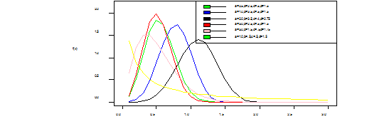
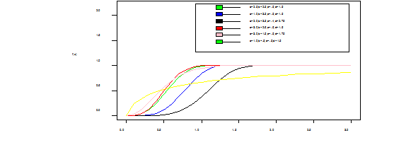
Figure 1 1a: Is the pdf of WIL which is unimodal and right skewed, 1b:Is the cdf of WIL which is J-shape which approaches each of the orthogonal axes asymptotically, 1c: Is the hazard function (bathtub curve) of WIL which is a decreasing failure rate function and lastly,1d: Is the survival function which shows that the probability that a subject will survive beyond time t, and its also a decreasing function.

Mixture representation

By inserting equations 2 and 1 in 1a we have

$f(x;\alpha \mathrm{,}\beta \mathrm{,}\gamma \mathrm{,}\lambda )=\alpha \beta \frac{\gamma \lambda }{x^2}{(1+\frac{\gamma }{x})}^{-(1+\lambda )}\frac{{\left({(1+\frac{\gamma }{x})}^{-\lambda }\right)}^{\beta -1}}{{(1-{(1+\frac{\gamma }{x})}^{-\lambda })}^{\beta +1}}\exp \{-\alpha {\left[\frac{{(1+\frac{\gamma }{x})}^{-\lambda }}{1-{(1+\frac{\gamma }{x})}^{-\lambda }}\right]}^{\beta }\}$ (11)

Let E be the last term of equation 11, by expanding E using power series

$E=\sum _{i=0}^{\infty }\frac{(-1{)}^i{\alpha }^i}{i!}\frac{{\left[{(1+\frac{\gamma }{x})}^{-\lambda }\right]}^{i\beta }}{{[1-{(1+\frac{\gamma }{x})}^{-\lambda }]}^{i\beta }}$

By inserting this expansion in equation 11 and after some algebra, we have

$f(x;\alpha \mathrm{,}\beta \mathrm{,}\gamma \mathrm{,}\lambda )=\sum _{i=0}^{\infty }\frac{(-1{)}^i{\alpha }^{i+1}}{i!}\beta \gamma \lambda {(1+\frac{\gamma }{x})}^{-\lambda \left[\beta \right(i+1\left)\right]-1}{[1-{(1+\frac{\gamma }{x})}^{-\lambda }]}^{-[\beta (i+1)+1]}$

let

After simplifications and some algebra, we have

$f(x;\alpha \mathrm{,}\beta \mathrm{,}\gamma \mathrm{,}\lambda )=\gamma \lambda \left[\beta \right(i+1)+j]\sum _{i\mathrm{,}j=0}^{\infty }{U}_{i\mathrm{,}j}\frac{{(1+\frac{\gamma }{x})}^{-\lambda \left[\beta \right(i+1)+j]-1}}{x^2}$ (12)

Where $U_{i\mathrm{,}j}=\frac{(-1{)}^i{\alpha }^{i+1}\beta }{i!j!}\frac{\Gamma \left(\beta \right(i+1)+j+1)}{\Gamma \left(\beta \right(i+1)+1)\beta (i+1)+j}$

Equation 12 reduces to

$f(x;\alpha \mathrm{,}\beta \mathrm{,}\gamma \mathrm{,}\lambda )=\sum _{i\mathrm{,}j=0}^{\infty }{U}_{i\mathrm{,}j}{h}_{\beta (i+1)+j}\left(x\right)$ (13)

Where $h_{\beta (i+1)+j}\left(x\right)=\gamma \lambda \left[\beta \right(i+1)+j]x^{-2}{(1+\frac{\gamma }{x})}^{-\lambda \left[\beta \right(i+1)+j]-1}$ is the Inverse

Lomax density. By integrating Equation 13, the cdf of X can be given in the mixture form

$F(x;\alpha \mathrm{,}\beta \mathrm{,}\gamma \mathrm{,}\lambda )=\sum _{i\mathrm{,}j=0}^{\infty }{U}_{i\mathrm{,}j}{H}_{\beta (i+1)+j}\left(x\right)$ (14)

Equation 13 above is the major result of this section.

Statistical Properties

Quantile function and median

Quantile function is used in drawing a sample from a particular distribution function. The quantile function of the WIL distribution is the inverse of 5 and is given by

$Qu=\frac{\gamma }{{[1-{\left(\frac{log(1-u)}{\alpha }\right)}^{\frac{-1}{\beta }}]}^{\frac{1}{\lambda }}-1}$ (15)

where u∼ uniform(0,1) and random numbers can easily be generated from the WIL distribution using $x=\frac{\gamma }{{[1-{\left(\frac{log(1-u)}{\alpha }\right)}^{\frac{-1}{\beta }}]}^{\frac{1}{\lambda }}-1}$

The median of the WIL distribution can be derived by setting u = 0.5 in 16 to be

$Median=\frac{\gamma }{{[1-{\left(\frac{log(0.5)}{\alpha }\right)}^{\frac{-1}{\beta }}]}^{\frac{1}{\lambda }}-1}$ (16) 

Moments

Must of the basic features and characteristics of a distribution can be studied through moments (for example kurtosis, tendency, skewness and dispersion). Theorem 4.1 If X∼WIL (α, β, γ, λ) then the r^th moments of X is given as

${\mu }_r^{\text{'}}=\sum _{i\mathrm{,}j=0}^{\infty }{U}_{i\mathrm{,}j}\lambda \left[\beta \right(i+1)+j]{\gamma }^{r}B(1-r\mathrm{,}\lambda \left(\beta \right(i+1)+j)+r)\mathrm{,}r=1,2,3,4\dots$ (17)

Proof.

Let start the prove with the well known definition of the r^th moment of the random variable X with probability density function f(x;α,β,γ,λ) given by

${\mu }_r^{\text{'}}\mathrm{<mo>=</mo>}{\displaystyle {\int }_0^{\infty }}{X}^{r}f\mathrm{<mo\; stretchy="false">(</mo>}x\mathrm{<mo\; stretchy="false">)</mo>}dx$

By substituting 13 in the above, we get

${\mu }_r^{\text{'}}=\sum _{i\mathrm{,}j=0}^{\infty }{U}_{i\mathrm{,}j}\gamma \lambda \left[\beta \right(i+1)+j]{\int }_0^{\infty }{X}^{r-2}{(1+\frac{\gamma }{x})}^{-\lambda \left[\beta \right(i+1)+j]-1}dx$

By letting $y\mathrm{<mo>=</mo>}\left(1+\frac{\gamma }{x}\right)$ and using the relation $B\left(p\mathrm{,}q\right)={\int }_0^{\infty }\frac{x^{m-1}}{(1+x{)}^{m+n}}dx$ as in

(4) and some simplifications, we have equation 17.

The mean and the variance of the WIL distribution are:

$E\left(X\right)={\mu }_1^{\text{'}}=\sum _{i\mathrm{,}j=0}^{\infty }{U}_{i\mathrm{,}j}\lambda \left[\beta \right(i+1)+j]\gamma B(\mathrm{0,}\lambda \left(\beta \right(i+1)+j)+1)$ (18)

$Var\mathrm{<mo\; stretchy="false">(</mo>}X\mathrm{<mo\; stretchy="false">)</mo><mo>=</mo>}E\mathrm{<mo\; stretchy="false">(</mo>}{X}^2\mathrm{<mo\; stretchy="false">)</mo>}-{\mathrm{<mo\; stretchy="false">[</mo>}E\mathrm{<mo\; stretchy="false">(</mo>}X\mathrm{<mo\; stretchy="false">)</mo><mo\; stretchy="false">]</mo>}}^2$

$=\sum _{i\mathrm{,}j=0}^{\infty }{U}_{i\mathrm{,}j}\lambda \left[\beta \right(i+1)+j]{\gamma }^{2}B(-\mathrm{1,}\lambda \left(\beta \right(i+1)+j)+2)$ $-{\left[\sum _{i\mathrm{,}j=0}^{\infty }{U}_{i\mathrm{,}j}\lambda \left[\beta \right(i+1)+j]\gamma B(\mathrm{0,}\lambda \left(\beta \right(i+1)+j)+1)\right]}^2$

Moment generating function

Theorem4.2 If X∼WIL (α,β,γ,λ) then the moment generating function (mgf) of X is given as

$M_x\mathrm{<mo\; stretchy="false">(</mo>}t\mathrm{<mo\; stretchy="false">)</mo><mo>=</mo>}{\displaystyle \sum _{r\mathrm{<mo>=</mo>0}}^{\infty }}\frac{t^r}{r\mathrm{<mo>!</mo>}}{\mu }_r^{\text{'}}$ (20)

Proof

By definition, the mgf of a random variable X with density f(x) is given

$M_x\mathrm{<mo\; stretchy="false">(</mo>}t\mathrm{<mo\; stretchy="false">)</mo><mo>=</mo>}{\displaystyle {\int }_{-\infty }^{\infty }}{e}^{tx}f\mathrm{<mo\; stretchy="false">(</mo>}x\mathrm{<mo\; stretchy="false">)</mo>}dx$

By substituting $e^{tx}={\sum }_{r=0}^{\infty }\frac{t(x{)}^r}{r!}$ in the above definition, we have

$M_x\left(t\right)={\sum }_{r=0}^{\infty }\frac{t^r}{r!}{x}^{r}f\left(x\right)dx={\sum }_{r=0}^{\infty }\frac{t^r}{r!}{\int }_{-\infty }^{\infty }{x}^{r}f\left(x\right)dx={\sum }_{r=0}^{\infty }\frac{t^r}{r!}{\mu }_r^{\text{'}}$ .

Order statistics

Order statistics are used in many areas of statistical theories and practices, for instance, detection of outlier in statistical quality control processes. In this section, we derive the closed form expressions for the pdf of the i^th order statistic of the Weibull Inverse Lomax distribution. Suppose is a random sample from a distribution with pdf f(x) and Let denotes the corresponding order statistics obtained from this sample. Then

$f_i{:}_n\left(x\right)=\frac{fx}{B(i\mathrm{,}n-i+1)}F{x}^{i-1}{[1-F(x\left)\right]}^{n-i}$ (21)

Where f(x) and F(x) are the pdf and cdf of Weibull Inverse Lomax distribution. Using the binomial expansion on

${\left[1-F\left(x\right)\right]}^n{}^{-1}$ ,

We have ${{[1-F\left(x\right)]}^n}^{-1}={\sum }_{k=0}^{\left(\infty \right)}(-1{)}^{k}F(x{)}^k$ by substituting back in the above equation

$f_{i:n}\left(x\right)=\frac{f\left(x\right)}{B(i\mathrm{,}n-i+1)}\sum _{k=0}^{\infty }(-1{)}^k\left(\begin{array}{c}n-i\\ k\end{array}\right)F(x{)}^{k}F(x{)}^{i-1}$ $=\frac{f\left(x\right)}{B(i\mathrm{,}n-i+1)}\sum _{k=0}^{\infty }(-1{)}^k\left(\begin{array}{c}n-i\\ k\end{array}\right)F(x{)}^{i+k-1}$ (22)

By expanding the last term and further simplifications and algebra, we have

$f_{i:n}\left(x\right)=\sum _{n\mathrm{,}p=0}^{\infty }{U}_{n\mathrm{,}p}{h}_{\beta (n+i+1)+j+p}\left(x\right)$ (23)

Where

$U_{n\mathrm{,}p}=\sum _{i\mathrm{,}j\mathrm{,}k\mathrm{,}m=0}^{\infty }\frac{(-1{)}^{i+k+m+n+p}{\alpha }^{i+n+1}\beta [i+k+m-1{]}^n\Gamma \left(\beta \right(i+1)+j+1)}{i!j!n!B(i\mathrm{,}n-i+1)\left(\beta \right(n+i+1)+j+p)\Gamma \left(\beta \right(i+1)+1)}$ $\times \left(\begin{array}{c}n-i\\ k\end{array}\right)\left(\begin{array}{c}n\beta \\ p\end{array}\right)\left(\begin{array}{c}i+k-1\\ m\end{array}\right)$

and

$h_{\beta (n+i+1)+j+p}\left(x\right)=\gamma \lambda \left[\beta \right(i+n+1)+j+p]x^{-2}{(1+\frac{\gamma }{x})}^{-\lambda \left[\beta \right(i+n+1)+j+p]}$

denotes the Inverse lomax density function with parameters $\gamma and\lambda \left[\beta \left(i+n+1\right)+j+p\right]$

Entropy

Rényi Entropy

The entropy of a random variable X is a measure of uncertain variation. we defined Rényi entropy by

$I\left(\zeta \right)\frac{1}{(1-\zeta )}log\left[{\int }_0^{\infty }{f}^{\zeta }\right(x\left)dx\mathrm{,}\right]\zeta >0 and \zeta \ne 1$

By replacing f(x) with equation (13) we have

$I\left(\zeta \right)=\frac{1}{(1-\zeta )}log\left[A{\int }_0^{\infty }{x}^{2\zeta }{(1+\frac{\gamma }{x})}^{-\lambda \zeta \left[\zeta \beta \right(I+1)+j]-1}dx\mathrm{,}\right]$ which can be reduced to

$I\left(\zeta \right)\frac{1}{(1-\zeta )}log\left[A{\int }_0^{\infty }{y}^{-\lambda \zeta \left[\zeta \beta \right(I+1)+j]-1}dy\mathrm{,}\right]$ (24)

Where

$A={\sum }_{i\mathrm{,}j=0}^{\infty }\frac{(-i{)}^i\zeta {\alpha }^{i+1}(\lambda \beta {)}^{\zeta }\zeta \beta (I+1)+j\Gamma \left(\zeta \beta \right(i+1)j+1)}{i!j!\Gamma \left(\zeta \beta \right(i+1)+1)\zeta \beta (i+1)+j}$

q-entropy

The q-entropy, say $E_q\mathrm{<mo\; stretchy="false">(</mo>}f\mathrm{<mo\; stretchy="false">)</mo>}$ is defined by $E_q\left(f\right)=\frac{1}{q-1}log[1-I_q(f\left)\right]$ ,

Where $I_q\left(f\right)={\int }_{\Re }{f}^q\left(x\right)dx\mathrm{,}q>0 and q\ne 1$ . From equation (24), we can obtain

$E_q\left(f\right)=\frac{1}{q-1}log[1-\left[C{\int }_0^{\infty }{y}^{-\lambda q\left[q\beta \right(I+1)+j]-1}dy\mathrm{,}\right]]$ (25)

Where $C={\sum }_{i\mathrm{,}j=0}^{\infty }\frac{(-i{)}^{i}q{\alpha }^{i+1}(\lambda \beta {)}^{q}q\beta (I+1)+j\Gamma \left(\zeta \beta \right(i+1)j+1)}{i!j!\Gamma \left(q\beta \right(i+1)+1)q\beta (i+1)+j}$

Estimation

Many parameter estimation techniques have been advocated in the literature, but the maximum likelihood method is the most frequently used. Furthermore, the MLEs have desirable properties and can be used to establish confidence intervals. The estimate of normality for these estimators is readily treated either numerically or analytically in the theory of large sample distribution. In this section, we determine the maximum likelihood estimates (MLEs) of the parameters of the Weibull Inverse Lomax distribution from complete samples only. Let $x_1,x_2,x_3,\mathrm{......},x_n$ be the observed values from the WIL distribution with parameter space $\theta ={\left(\alpha ,\beta ,\gamma ,\lambda \right)}^T$ be the $r\times 1$ parameter vector. The log-likelihood function for θ is given by

$l\left(\theta \right)=nlog\left(\alpha \beta \gamma \lambda \right)-2\sum _{i=1}^{n}log{x}_i-(1+\lambda )\sum _{i=1}^{n}log(1+\frac{\gamma }{x_i})+(\beta -1)\sum _{i=1}^{n}log(1+\frac{\gamma }{x_i}{)}^{-\lambda }$ $-(\beta +1)\sum _{i=1}^{n}log(1-(1+\frac{\gamma }{x_i}\left)\right)-\alpha \sum _{i=1}^n{\left[\frac{(1+\frac{\gamma }{x_i})}{1-(1+\frac{\gamma }{x_i})}\right]}^{\beta }$ (26)

Differentiating $l\left(\theta \right)$ with respect to each parameter $\alpha ,\beta ,\gamma and\lambda$ and setting the result equals to zero, we obtain maximum likelihood estimates (MLEs). The partial derivatives of $l\left(\theta \right)$ with respect to each parameter or the score function is given by:

$W_n\mathrm{<mo\; stretchy="false">(</mo>}\theta \mathrm{<mo\; stretchy="false">)</mo><mo>=</mo>}\left(\frac{\partial l}{\partial \alpha }\mathrm{,}\frac{\partial l}{\partial \beta }\mathrm{,}\frac{\partial l}{\partial \gamma }\mathrm{,}\frac{\partial l}{\partial \lambda }\right)$

where

$\frac{\partial l}{\partial \alpha }=\frac{n}{\alpha }+\sum _{i=1}^n{[1-(1+\frac{\gamma }{x}{)}^{\lambda }]}^{-\beta }{\alpha }^{\beta -1}$ (27)

$\frac{\partial l}{\partial \beta }=\frac{n}{\beta }-\lambda \sum _{i=1}^{n}log(1+\frac{\gamma }{x_i})-\sum _{i=1}^{n}log[1-(1+\frac{\gamma }{x_i}{)}^{-\lambda }]+\alpha \sum _{i=1}^n{[1-(1+\frac{\gamma }{x_i}{)}^{\lambda }]}^{-\beta }$ $\times log\left(\frac{\alpha }{{\displaystyle \sum _{i=1}^n[1-(1+\frac{\gamma }{x_i}{)}^{\lambda }]}}\right)$ (28)

$\frac{\partial l}{\partial \gamma }=\frac{n}{\gamma }-(\lambda \beta +\underset{i=1}{\overset{n}{1)\sum (}}{x}_i+\gamma {)}^{-1}-(\beta +\underset{i=1}{\overset{n}{1)\sum }}\frac{\lambda }{(x_i+\gamma )\left(\right(1+\frac{\gamma }{x_i}{)}^{\lambda }-1)}$ $+\alpha \sum _{i=1}^n\beta \lambda (1+\frac{\gamma }{x_i}{)}^{\lambda }{[1-(1+\frac{\gamma }{x}{)}^{\lambda }]}^{-\beta -1}(\gamma +x_i{)}^{-1}$ (29)

$\frac{\partial l}{\partial \lambda }=\frac{n}{\lambda }-\beta \sum _{i=1}^{n}log(1+\frac{\gamma }{x_i})-(\beta +1)\sum _{i=1}^{n}log(1+\frac{\gamma }{x_i}){\left[\right(1+\frac{\gamma }{x_i}{)}^{\lambda }-1]}^{-1}$ $+\alpha \sum _{i=1}^n\beta {(1+\frac{\gamma }{x_i})}^{\lambda }log(1+\frac{\gamma }{x_i}){[1-(1+\frac{\gamma }{x_i})]}^{-\beta -1}$ (30)

In this section, we illustrate the applicability of the WIL distribution to the monthly remission of the 128 bladder cancer patients as reported by Maxwell et al.²³ We estimated the parameters of each model by the method of Maximum Likelihood Estimation (MLE) using Simulated ANNealing (SANN) method. The goodness of fit statistics used in comparing the performances are Akaike Information Criterion AIC and Bayesian Information Criterion. Smaller values of the AIC and BIC statistics indicates better model fittings. Throughout the analysis, we used log-likelihood (- ll) value to derive the AIC and BIC by using the following relations: AIC = −2(−ll) + 2p and BIC = −2(−ll) + plog(n) where p is the number of parameters and n is the sample size. The data is given below:

0.08, 2.09, 3.48, 4.87, 6.94, 8.66, 13.11, 23.63, 0.20, 2.23, 3.52, 4.98, 6.97,

9.02, 13.29, 0.40, 2.26, 3.57, 5.06, 7.09, 9.22, 13.80, 25.74, 0.50, 2.46, 3.64,

5.09, 7.26, 9.47, 14.24, 25.82, 0.51, 2.54, 3.70, 5.17, 7.28, 9.74, 14.76, 26.31,

0.81, 2.62, 3.82, 5.32, 7.32, 10.06, 14.77, 32.15, 2.64, 3.88, 5.32, 7.39, 10.34,

14.83, 34.26, 0.90, 2.69, 4.18, 5.34, 7.59, 10.66, 15.96, 36.66, 1.05, 2.69, 4.23 , 5.41, 7.62, 10.75, 16.62, 43.01, 1.19, 2.75, 4.26, 5.41, 7.63, 17.12, 46.12, 1.26 ,

2.83, 4.33, 5.49, 7.66, 11.25, 17.14, 79.05, 1.35, 2.87, 5.62, 7.87, 11.64, 17.36,

1.40, 3.02, 4.34, 5.71, 7.93, 11.79, 18.10, 1.46, 4.40, 5.85, 8.26, 11.98, 19.13 , 1.76, 3.25, 4.50, 6.25, 8.37, 12.02, 2.02, 3.31, 4.51, 6.54, 8.53, 12.03, 20.28 ,

2.02, 3.36, 6.76, 12.07, 21.73, 2.07, 3.36, 6.93, 8.65, 12.63, 22.69. Firstly, it is usual to begin the analysis with plots of empirical distribution function and the histogram (density plot), as in figure 2a and Table 1. The left-hand plot is the histogram on a density scale and the right-hand plot is the empirical cumulative distribution function (CDF). While figure 2b is the skewness-kurtosis plot as proposed by Cullen & Aral et al.,^24,25 in which the values for common distributions are displayed in order to guide the researcher for the choice of distributions to fit the data set. As in our case, Weibull distribution is suggested. For this data, we fit Weibull-Inverse Lomax (WIL) distribution defined in equation (6). Its fit is also compared with the Weibull-Lomax distribution by Tahir et al.,⁹ Weibull-Frechet by Atify et al.,¹¹ Odd generalized exponential inverse lomax distribution by Falgore et al.,¹⁸ and Inverse lomax distribution as in Rahman et al.¹⁵ with the pdfs given below:

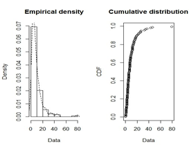
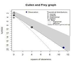
Figure 2 2a is the empirical and cdf plots of the data set and 2b is the Skewness-kurtosis plot for a bladder cancer patients data set.

$f\mathrm{<mo\; stretchy="false">(</mo>}x\mathrm{<mo>;</mo>}\alpha \mathrm{,}\beta \mathrm{,}\gamma \mathrm{,}\lambda \mathrm{<mo\; stretchy="false">)</mo><mo>=</mo>}\frac{\gamma \lambda \alpha }{\beta }{\left[1+\left(\frac{x}{\beta }\right)\right]}^{\lambda \alpha -1}{\left\{1-{\left[1+\left(\frac{x}{\beta }\right)\right]}^{-\alpha }\right\}}^{\lambda -1}\exp \left\{-\alpha {\left[{\left(1+\frac{x}{\beta }\right)}^{\alpha }-1\right]}^{\lambda }\right\}$ $\times exp\left\{-\gamma {\left(exp\left\{{\left(\frac{\alpha }{x}\right)}^{\beta }\right\}-1\right)}^{-\lambda }\right\}$

$f\mathrm{<mo\; stretchy="false">(</mo>}x\mathrm{<mo>;</mo>}\alpha \mathrm{,}\beta \mathrm{,}\gamma \mathrm{,}\lambda \mathrm{<mo\; stretchy="false">)</mo><mo>=</mo>}\alpha \beta \gamma \lambda {\left(1+\left(\frac{\beta }{x}\right)\right)}^{\alpha -1}exp\left\{\frac{\lambda }{1-{\left(\frac{\beta }{x}+1\right)}^{\alpha }}\right\}{\left\{1-exp\left\{\frac{\lambda }{1-{\left(\frac{\beta }{x}+1\right)}^{\alpha }}\right\}\right\}}^{\alpha -1}\times {\left[x^2{\left[{\left(\frac{\beta }{x}+1\right)}^{\alpha }-1\right]}^2\right]}^{-1}$

for $0<x<\infty and\alpha ,\beta ,\gamma and \lambda >0.$

We have successfully proposed a flexible WIL distribution by extending the weibull-G family of Bourguignon et al.⁶ We have derived and studied some properties of this distribution including mean, variance, quantile, moments, moment generating function, entropies and order statistics. The parameters of the distribution were estimated by employing the method of maximum likelihood. Finally, an application of the WIL distribution to real data set is presented to show the importance and flexibility of the distribution. The AIC and BIC in Table 2 shows that the WIL distribution is the best model fitted.

No funding for this project and also no conflicts of interest among the authors.

1. Afify AZ, Nofal ZM, Yousof HM, et al. The transmuted weibull lomax distribution: properties and application. Pakistan Journal of Statistics and Operation Research. 2015;11(1):135–152.
2. Alizadeh M, Tahir M, Cordeiro GM, et al. The kumaraswamy marshal-olkin family of distributions. Journal of the Egyptian Mathematical Society. 2015;23(3):546–557.
3. Cordeiro GM, Ortega EM, Popovic BV, et al. The lomax generator of distributions: Properties, minification process and regression model. Applied Mathematics and Computation, 2014;247:465–486.
4. Oguntunde P, Balogun O, Okagbue H, et al. The weibull-exponential distribution: Its properties and applications. Journal of Applied Sciences, 2015;15(11):1305–1311.
5. Bourguignon M, Silva RB, Zea LM, et al. The kumaraswamy pareto distribution. Journal of Statistical Theory and Applications. 2013;12(2):129–144.
6. Bourguignon M, Silva RB, Cordeiro GM. The weibull-g family of probability distributions. Journal of Data Science. 2014;12(1):53–68.
7. Tahir M, Cordeiro GM, Mansoor M, et al. The weibull–dagum distribution: Properties and applications. Communications in Statistics-Theory and Methods. 2016;45(24):7376–7398.
8. Nofal ZM, Afify AZ, Yousof HM, et al. The generalized transmuted-g family of distributions. Communications in Statistics-Theory and Methods. 2017;46(8):4119–4136.
9. Tahir M, Cordeiro GM, Mansoor M, et al. The weibull-lomax distribution: properties and applications. Hacettepe Journal of Mathematics and Statistics. 2015;44(2):461–480.
10. Merovci F, Elbatal I. Weibull rayleigh distribution: Theory and applications. Applied Mathematics & Information Sciences. 2015;9(4):2127.
11. Afify A, Yousof H, Cordeiro G, et al. The weibull fréchet distribution and its applications. Journal of Applied Statistics. 2016;43(14):2608–2626.
12. Yousof HM, Rasekhi M, Afify A. et al. The beta weibull-g family of distributions: Theory, characterizations and applications. Pakistan Journal of Statistics. 2017;33(2).
13. Kleiber C, Kotz S. Statistical size distributions in economics and actuarial sciences. John Wiley & Sons.2003;470.
14. Kleiber C. Lorenz ordering of order statistics from log-logistic and related distributions. Journal of Statistical Planning and Inference. 2004;120(1-2):13–19.
15. Rahman J, Aslam M, Ali S. Estimation and prediction of inverse lomax model via bayesian approach. Caspian Journal of Applied Sciences Research. 2013;2(3):43–56.
16. Yadav AS, Singh SK, Singh U. On hybrid censored inverse lomax distribution: Application to the survival data. Statistica. 2016;76(2):185–203.
17. Reyad HM, Othman SA. E-bayesian estimation of two component mixture of inverse lomax distribution based on type-i censoring scheme. Journal of Advances in Mathematics and Computer Science. 2018;26:1–22.
18. Falgore JY, Aliyu Y, Umar AA, et al. Odd generalized exponential-inverse lomax distribution: Properties and application. Journal of the Nigerian association of Mathematical physics, volume 47:147-156.
19. Maxwell O, Friday A, Chukwudike N, et al. A theoretical analysis of the odd generalized exponentiated inverse lomax distribution. Biom Biostat Int J. 2019b;8(1):17–22.
20. Yakubu A, Doguwa SI. On the properties of the weibullburr iii distribution and its application to uncensored and censored survival data. CBN Journal of Applied Statistics, 2017;8(2):91–116.
21. Cooray K. Generalization of the weibull distribution: the odd weibull family. Statistical Modelling. 2006;6(3):265–277.
22. Gupta RD, Kundu D. Theory & methods: Generalized exponential distributions. Australian & New Zealand Journal of Statistics. 1999;41(2):173–188.
23. Maxwell O, Chukwu AU, Oyamakin OS, et al. The marshall-olkin inverse lomax distribution (mo-ild) with application on cancer stem cell. Journal of Advances in Mathematics and Computer Science. 2019a;1–12.
24. Cullen AC, Frey HC, Frey CH. Probabilistic techniques in exposure assessment: a handbook for dealing with variability and uncertainty in models and inputs. Springer Science & Business Media. 1999.
25. Aral A, Gupta V. (p,q)-type beta functions of second kind. Advances in Operator Theory. 2016;1(1):134–146.