Research Article Volume 6 Issue 4
The odd log-logistic generalized gamma model: properties, applications, classical and bayesian approach
Fábio Prataviera,1 Gauss M Cordeiro,2 Adriano K Suzuki,3 Edwin MM Ortega4
1Departamento de Ciências Exatas, Universidade de São Paulo, Brazil
2Departamento de Estat´ıstica, Universidade Federal de Pernambuco, Brazil
3Departamento de Matemática Aplicada e Estat´ıstica, Universidade de São Paulo, Brazil
4Departamento de Ciências Exatas, Universidade de São Paulo, Brazil
Correspondence: Edwin M. M. Ortega, Departamento de Ciências Exatas, Universidade de São Paulo, Piracicaba, SP, Brazil
Received: September 23, 2017 | Published: October 27, 2017
Citation: Prataviera, F, Cordeiro GM, Suzuki AK, et al. The odd log-logistic generalized gamma model: properties, applications, classical and bayesian approach. Biom Biostat Int J. 2017;6(4):388-405. DOI: 10.15406/bbij.2017.06.00174
Download PDF
Abstract
We propose a new lifetime model called the odd log-logistic generalized gamma distribution that can be easily interpreted. Some of its special models are discussed. We obtain general mathematical properties of this distribution including the ordinary moments, and quantile functions. We discuss parameter estimation by the maximum likelihood method and a Bayesian approach, where Gibbs algorithms along with metropolis steps are used to obtain the posterior summaries of interest for survival data with right censoring. Further, for different parameter settings, sample sizes and censoring percentages, we perform various simulations and evaluate the behavior of the estimators. The potentiality of the new distribution is proved by means of two real data sets. In fact, the new distribution can produce better fits than some well-known distributions.
Keywords:censored data, exponentiated distribution, generalized gamma distribution, moments, survival analysis
Introducton
The statistics literature is filled with hundreds of continuous univariate distributions. Recent developments focus on new techniques for building meaningful models. More recently, several methods of introducing one or more parameters to generate new distributions have been proposed. Among these methods, the compounding of some discrete and important lifetime distributions has been in the vanguard of lifetime modeling. So, several families of distributions were investigated by compounding some useful lifetime and truncated discrete distributions. The log-logistic (LL) distribution with a shape parameter
is a useful model for survival analysis and it is an alternative to the log-normal distribution. Unlike the more commonly used Weibull distribution, the LL distribution has a non-monotonic hazard rate function (hrf), which makes it suitable for modeling cancer survival data. For
, the hrf is unimodal and when
, the hazard decreases monotonically. The fact that its cumulative distribution function (cdf) has a closed-form is particularly useful for analysis of survival data with censoring.
The odd log-logistic (OLL) family of distributions was pioneered by Gleaton and Lynch;1 they called this family the generalized log-logistic (GLL) family. Recently, Braga et al.2 studied the odd log-logistic normal distribution, da Cruz et al.3 proposed the odd log-logistic Weibull distribution and Cordeiro et al.2 proposed the beta odd log-logistic generalized family. We develop a similar methodology to propose a new model based on the generalized gamma (GG) distribution. The GG distribution plays a very important role in statistical inferential problems. When modeling monotone hazard rates, the Weibull distribution may be an initial choice because of its negatively and positively skewed density shapes. However, the Weibull distribution does not provide a reasonable parametric fit for modeling phenomenon with bathtub shaped and unimodal failure rates, which are common in biological and reliability studies. Alternatively, other extensions of the GG distribution were developed for modeling lifetime data. For example, Cordeiro et al.4 defined the exponentiated generalized gamma with applications, Pascoa et al.5 introduced the Kumaraswamy generalized gamma distribution, Ortega et al.6 proposed the generalized gamma geometric distribution, Cordeiro et al.7 studied the beta generalized gamma distribution and, more recently, Lucena et al.8 defines the transmuted generalized gamma distribution and Silva et al.9 proposed the generalized gamma power series class.
Given a continuous baseline cdf
with a parameter vector
, the cdf of the odd log-logistic-G (“OLL-G” for short) distribution with an extra shape parameter
is defined by
(1)
We can write
and
So, the parameter
represents the quotient of the log odds ratio for the generated and baseline distributions. We note that there is no complicated function in equation (1) in contrast with the beta generalized family (Eugene et al.,10), which includes two extra parameters and also involves the beta incomplete function. The baseline cdf
is clearly a special case of (1) when
. If
, it becomes the LL distribution. Several distributions can be generated from equation (1). For example, the odd log-logistic Fréchet and odd log-logistic gamma distributions are obtained by taking
to be the Fréchet and gamma cumulative distributions, respectively. The probability density function (pdf) of the new family is given by
(2)
The OLL-G family of densities (2) allows for greater flexibility of its tails and can be widely applied in many areas of engineering and biology. We can study some of its mathematical properties because it extends several well-known distributions.
The inferential part of this model is carried out using the asymptotic distribution of the maximum likelihood estimators (MLEs), which in situations when the sample size is small or moderate, might lead to poor inference on the model parameters. Hence, in this paper, we also explore the Markov Chain Monte Carlo (MCMC) techniques to develop a Bayesian inference as an alternative analysis for the model. So, we discuss the inference aspects of the OLL-G model following both a classical and a Bayesian approach.
The rest of the paper is organized as follows. In Section 2, we define the odd log-logistic generalized gamma (OLLGG) distribution and present some special cases. Section 3 provides a useful linear representation for the OLLGG density function. We derive in Section 4 some structural properties of the new distribution. Considering censored data, we adopt a classic analysis for the parameters of the model in Section 5. In Section 6, the Bayesian approach is considered using MCMC with Metropolis-Hasting algorithms steps to obtain the posterior summaries of interest. In Section 7, we present results from various simulation studies displayed graphically and commented. Two applications to real data are performed in Section 8. Some concluding remarks are given in Section 9.
The OLLGG distribution
The gamma distribution is the most popular model for analyzing skewed data. The generalized gamma distribution (GG) was introduced by Stacy11 and includes as special models: the exponential, Weibull, gamma and Rayleigh distributions, among others. It is suitable for modeling data with different forms of the hazard rate function (hrf): increasing, decreasing, bathtub and unimodal. This characteristic is useful for estimating individual hrfs and both relative hazards and relative times. The GG distribution has been used in several research areas such as engineering, hydrology and survival analysis.
The cdf and pdf of the
distribution (Stacy,10) are given by
(3)
(4)
where
is the incomplete gamma function and
is the gamma function. Basic properties of the GG distribution are given by Stacy and Mihram12 and Lawless.13 The OLLGG distribution (for t > 0) is defined by substituting
in equations (1) and (2), respectively. Hence, its density function with four positive parameters
and
has the form
(5)
where α is a scale parameter and the other positive parameters τ,
and
are shape parameters. One major benefit of (5) is its ability of fitting skewed data that can not be properly fitted by existing distributions. The OLLGG density allows for greater flexibility of its tails and can be widely applied in many areas of engineering and biology.
The Weibull and GG distributions are the most important sub-models of (5) for
and
, respectively. The OLLGG distribution approaches the log-normal (LN) distribution when
and
. Other sub-models are listed in Table 2: OLL-Gamma, OLL-Chi-Square, OLL-Exponential, OLL-Weibull, OLL-Rayleigh, OLL-Maxwell, OLL-Folded normal, among others.
Distribution |
|
|
|
|
OLL-Gamma |
|
1 |
|
|
OLL-Weibull |
|
|
1 |
|
OLL-Exponential |
|
1 |
1 |
|
OLL-Chi-square |
2 |
1 |
|
|
OLL-Chi |
|
2 |
|
|
OLL-Rayleigh |
|
2 |
1 |
|
OLL-Maxwell |
|
2 |
|
|
OLL-Folded normal |
|
2 |
|
|
OLL-Circular normal |
|
2 |
1 |
|
OLL-Spherical Normal |
|
2 |
|
|
Table 1 Some new OLL-G sub-models
If
is a random variable with density function (5), we write
. The survival and hazard rate functions corresponding to (5) are
(6)
(7)
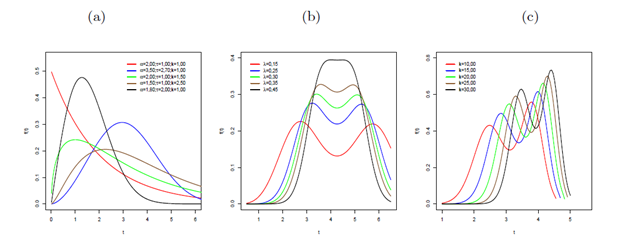
respectively. Plots of the OLLGG density function for selected parameter values are given in Figure 1. We note that the OLLGG density function can be symmetrical, left-skewed, right-skewed, unimodal and bimodal shaped.
The hrf (7) is quite flexible for modeling survival data as indicated by the plots for selected parameter values in Figure 2. The hrf can be increasing, decreasing, unimodal, bathtub and have other forms.

Figure 1 Plots of the OLLGG density function for some parameter values. (a) Fixed
. (b) Fixed
,
and
. (c) Fixed
,
and
.

Figure 2 The OLLGG hrf. (a) Bathtub. (b) Unimodal. (c) Increasing, decreasing and other forms.
The OLLGG model is easily simulated by inverting (1) as follows:
, (8)
where
has a uniform
distribution and
is the baseline quantile function
(qf).
Some properties of the OLLGG distribution are:
If
If
So, the new distribution is closed under power transformation.
Linear representation for the OLLGG distribution
First, we define the exponentiated-generalized gamma (“Exp-GG”) distribution, say
with power parameter
, if
has cdf and pdf given by
and
respectively. In a general context, the properties of the exponentiated-G (Exp-G) distributions have been studied by several authors for some baseline G models, see Mudholkar and Srivastava14 and Mudholkar et al.15 for exponentiated Weibull, Nadarajah16 for exponentiated Gumbel, Shirke and Kakade.17 for exponentiated log-normal and Nadarajah and Gupta18 for exponentiated gamma distributions. See, also, Nadarajah and Kotz,19 among others.
First, we obtain an expansion for
using a power series for
(
real)
(9)
where
For any real
, we consider the generalized binomial expansion
(10)
Inserting (9) and (10) in equation (1), we obtain
where
for
The ratio of the two power series can be expressed as
(11)
where
and the coefficients
’s (for
) are determined from the recurrence equation
The pdf of
is obtaining by differentiating (11) as
(12)
where
is the Exp-GG density function with power parameter
.
For
, we can write
(13)
where
By application of an equation in Section 0.314 of Gradshteyn and Ryzhik20 for a power series raised to a power, we obtain for any
positive integer
(14)
where the coefficients
satisfy the recurrence relation
(15)
and
. The coefficient
can be expressed explicitly from
and then from
, although it is not necessary for programming numerically our expansions using any software with numerical facilities.
Further, using equation (14), we can write (for
)
(16)
where the coefficients
are determined from (15) with
Based upon equation (16), we can write the Exp-GG density (for
) from (13) as
The last density can be expressed in terms of the GG density functions. By noting the form of (4), we can write (for
)
(17)
where
is the GG density function with parameters
and
and
(18)
For
, we have from (13)
Combining the result (17) (for
) and that one for
, we can write
in (12) as
(19)
Equation (19) reveals that the OLLGG density function is a linear combination of Exp-GG densities. Hence, some mathematical properties of the OLLGG distribution can follow directly from those properties of the GG distribution. For example, the ordinary, central, fac¬torial moments and the moment generating function (mgf) of the proposed distribution can be obtained from the same weighted infinite linear combination of the corresponding quantities for the GG distribution. This equation is the main result of this section.
Mathematical properties
Some of the most important features and characteristics of a distribution can be studied through moments (e.g., tendency, dispersion, skewness and kurtosis). In this section, we give two different expansions for calculating the moments of the EGG distribution.
First, we obtain an infinite sum representation for the
th ordinary moment
of the EGG distribution based on the equation (19). The
th moment of the
distribution is well known to be
Equation (19) then immediately gives
(20)
Equation (20) reveals that the moment
does have the inconvenient of depending on the quantities
given by (18).
We now derive another infinite sum representation for
by computing the
th moment directly without requiring the quantities
. We readily obtain
and then
gives
Using expansion (16) for
leads to
Inserting the last equation in the expression for
and interchanging terms, we obtain
(21)
where
.
For calculating the last integral, the series expansion (16) for the incomplete gamma function gives
Now this integral can be obtained from equations (24) and (25) of Nadarajah21 in terms of the Lauricella function of type A (Exton,22 Aarts,23) defined by
where
is the ascending factorial defined by (with the convention that
)
Numerical routines for the direct computation of the Lauricella function of type A are available, see Exton22 and Mathematica (Trott,24). We obtain
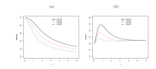
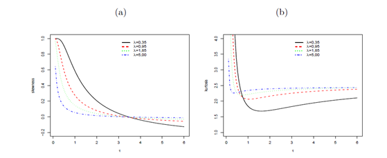
(22) Hence, as an alternative way to equation (20), the rth moment of the EGG distribution follows from both formulae (21) and (22) as an infinite weighted sum of the Lauricella functions of type A. In Figures 3 and 3, we display plots of the skewness and kurtosis the OLGG distribution for some parameter values.
Maximum likelihood estimation
Let Ti be a random variable following (5) with the vector of parameters
. The data encountered in survival analysis and reliability studies are often censored. A very simple random censoring mechanism that is often realistic is one in which each individual
is assumed to have a lifetime
and a censoring time
, where
and
are independent random variables. Suppose that the data consist of n independent observations
for

Figure 3 Skewness and kurtosis of the OLLGG distribution as a function of
for some values of
with
and
.

Figure 4 Skewness and kurtosis of the OLLGG distribution as a function of
for some values of
with
and
.
The distribution of
does not depend on any of the unknown parameters of
. Parametric inference for such data are usually based on likelihood methods and their asymptotic theory. The censored log-likelihood
for the model parameters is given by
(23)
Where
,
is the number of failures and
and
denote the uncensored and censored sets of observations, respectively.
The score components corresponding to the parameters in
are:
and
Where
is the digamma function and
.
The
of
can be obtained numerically from the nonlinear equations
For interval estimation and hypothesis tests on the model parameters, we require the
unit observed information matrix
, whose elements are evaluated numerically. Under general regularity conditions, the asymptotic distribution of
is
, where
is the expected information matrix. This matrix can be replaced by
, i.e., the observed information matrix evaluated at
. The multivariate normal
distribution can be used to construct approximate confidence intervals for the individual parameters. Further, the likelihood ratio (LR) statistic can be adopted for comparing this distribution with some of its special models. We can compute the maximum values of the unrestricted and restricted log-likelihoods to construct LR statistics for testing some sub-models of the OLLGG distribution. For example, the test of
versus
is not true is equivalent to compare the OLLGG and GG distributions and the LR statistic reduces to
where
, and
are the MLEs under H and
and
are the estimates under
.
Bayesian inference
In this section we briefly discuss the inference from a Bayesian viewpoint. We making a change in the parameters to
, so that the parameter space is transformed into
(necessary for the work with the proposed Gaussian densities). We assume that
are prior independent, that is,
where
and
denotes the normal distribution with mean
and variance
. All the hyper-parameters
have been specified to express non-informative priors.
Regarding the Jacobian of this transformation, our joint posterior density (or target density) reduces to
(25)
where
is the likelihood function.
This joint posterior density is analytically intractable. Therefore, we based our inference on the MCMC simulation methods. No closed-form is available for any of the full conditional distributions necessary for the implementation of the Gibbs sampler. Then, we have resorted to the Metropolis–Hastings algorithm. To implement this algorithm, we proceed as follows:
(1) Start with any point
and stage indicator
;
(2) Generate a point
according to the transitional kernel
, where
is the covariance matrix of
, which is the same in any stage;
(3) Update
′ with probability
, or keep
;
(4) Repeat steps (2) and (3) by increasing the stage indicator until the process has reached a stationary distribution.
In this scheme, we consider 30,000 sample burn-in, and we use every tenth sample from the 200,000 MCMC posterior samples to reduce the autocorrelations and yield better convergence results, thus obtaining an effective sample of size 20,000 from which the posterior is based on. We monitor the convergence of the Metropolis-Hasting algorithm using the method proposed by Geweke (1992), as well as trace plots. All computations are performed in the
software (
Development Core Team, 2011).
Bayesian model comparison
In the literature, a variety of Bayesian methodologies can be applied for comparing of several competing models for a given data set and selection of the best one to fit the data. In this paper, we use the deviance information criterion (DIC) proposed by Spiegelhalter et al.,25 the expected Akaike information criterion (EAIC)given by Brooks,26 and the expected Bayesian (or Schwarz) information criterion (EBIC) discussed by Carlin and Louis.27
They are based on the posterior mean of the deviance, which can be approximated by
. The DIC criterion can be estimated using the MCMC output by
, where ρD is the effective number of parameters given by
is the deviance evaluated at the posterior mean. Similarly, the EAIC and EBIC criteria can be estimated by means of
and
is the number of the model parameters.
Simulation study
We evaluate some properties of the MLEs using the classical and Bayesian analysis by means of a simulation study. We simulate the OLLGG distribution considering modality form from equation (8) by using a random variable U having a uniform distribution in (0, 1).
We take n=50, 150 and 350 and, for each replication, we calculate the MLEs
. We repeat this process 1, 000 times and determine the average estimates (AEs), biases and means squared errors (MSEs). In this study, we consider two scenarios. In the first scenario, we take
In the second scenario, we use the values fitted in the adjustment to the temperature data set in Section 8
. The estimates of
are determined by solving the nonlinear equations
. The results of the Monte Carlo study under maximum likelihood and Bayesian estimation are given in Tables 2 and 3, respectively. They indicate that the MSEs of the MLEs of
decay toward zero as the sample size increases, as expected under first-order asymptotic theory. The same results are obtained using the Bayesian approach. In Figures 5 and 6, we present the estimated densities based on 1,000 samples of the AEs of the parameters
, respectively and n = 50, 150 and 350 for both scenarios. These plots are in agreement with the first-order asymptotic theory for the MLEs and reveal a fast convergence even for small sample sizes.
Simulation study of random censored values
Similarly, we also consider a simulation study in the presence of censored data. The censoring times
are sampled from the uniform distribution in the interval
denotes the proportion of censored observations. In this study, the proportions of censored observations are approximately equal to 10% and 30%. In this scenario, we take the values of the parameters as
. Table 4 lists the averages of the MLEs (Mean) and the MSEs. The figures in this table indicate that the MSEs increase when the censoring percentage increases. Further, the MSEs of the MLEs of
decay toward zero as the sample size increases, as expected under first-order asymptotic theory.
Table 5 lists the posterior means (Mean) and the MSEs. We can note that increasing the sample size and decreasing the percentage of censure, the estimates are closer to the true values with lower MSEs.
Scenario 1 |
|
Parameters |
AEs |
Biases |
MSEs |
50 |
|
2.0404 |
-0.0404 |
0.1984 |
|
5.3257 |
-0.3257 |
1.8523 |
|
10.7653 |
-0.7653 |
2.9000 |
|
0.1708 |
-0.0208 |
0.0115 |
150 |
|
2.0393 |
-0.0393 |
0.0242 |
|
5.1585 |
-0.1585 |
0.2070 |
|
9.8491 |
0.1509 |
1.9955 |
|
0.1528 |
-0.0028 |
0.0011 |
350 |
|
2.0065 |
-0.0065 |
0.0024 |
|
5.0417 |
-0.0417 |
0.0276 |
|
10.012 |
-0.0012 |
0.2220 |
|
0.1511 |
-0.0011 |
0.0001 |
Scenario 2 |
|
Parameters |
AEs |
Biases |
MSEs |
50 |
|
21.1422 |
0.1489 |
7.7557 |
|
15.5491 |
-2.483 |
64.7128 |
|
4.5288 |
-1.6533 |
22.2571 |
|
0.3400 |
-0.0518 |
0.0685 |
150 |
|
21.3407 |
-0.0496 |
2.1903 |
τ |
13.8973 |
-0.8312 |
9.9415 |
|
3.2666 |
-0.3911 |
3.3779 |
|
0.3060 |
-0.0178 |
0.0167 |
350 |
|
21.2908 |
0.0003 |
0.8393 |
τ |
13.3138 |
-0.2477 |
3.0814 |
|
3.0593 |
-0.1838 |
1.2018 |
|
0.2956 |
-0.0074 |
0.0058 |
Table 2 AEs, biases and MSEs for the estimates of the OLLGG parameters
In Figures 7 and 8, we present the estimated densities based on 1,000 samples of the AEs of the parameters
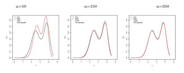
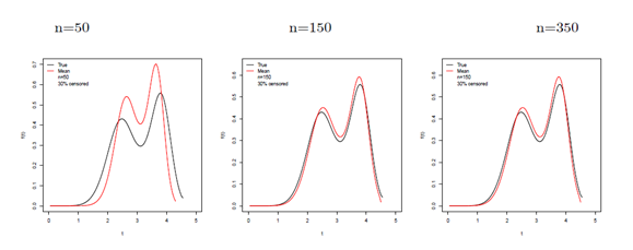
respectively, and n = 50, 150 and 350 for both scenarios with 10% and 30% of censored. These plots are in agreement with the first-order asymptotic theory for the MLEs and indicate a fast convergence even for small sample sizes and considering censored data.
Applications
In this section, we provide two applications to real data to prove empirically the flexibility of the OLLG model. The computations are performed using the R software and NLMixed procedure in SAS. In the first application, we give an application for bimodal data comparing the OLLGG, GG and Weibull models. In the second application, we prove the usefulness of the new distribution for censored data.
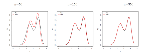
Figure 5 Some OLLGG density functions at the true parameter values and at the AEs for scenario 1.
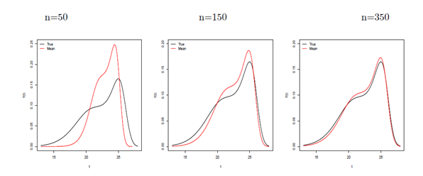
Figure 6 Some OLLGG density functions at the true parameter values and at the AEs for scenario 2.
Temperature data
The first data set refers to daily temperatures
in the period from January 1 to December 31, 2011 in the city of Piracicaba obtained from the Department of Biosystems Engi-neering of the Luiz de Queiroz Superior School of Agriculture (ESALQ), part of the University of São Paulo (USP).
We show the superiority of the OLLGG distribution as compared to some of its sub-mo¬dels and also to the following non-nested models: the exponentiated generalized gamma (EGG) proposed by Cordeiro et al.28 and beta Weibull (BW) distributions. The BW cdf (Famoye et al.,29) is given by
Scenario 1 |
|
Parameters |
Means |
Biases |
MSEs |
50 |
|
1.8130 |
0.1870 |
0.0703 |
|
4.1719 |
0.8281 |
1.1152 |
|
9.9011 |
0.0989 |
0.0601 |
|
0.2795 |
-0.1295 |
0.0319 |
150 |
|
1.8891 |
0.1109 |
0.0240 |
|
4.4648 |
0.5352 |
0.4132 |
|
9.9893 |
0.0107 |
0.0824 |
|
0.2005 |
-0.0505 |
0.0031 |
350 |
|
1.9283 |
0.0717 |
0.0128 |
|
4.6425 |
0.3575 |
0.2232 |
|
9.9929 |
0.0071 |
0.0913 |
|
0.1812 |
-0.0312 |
0.0014 |
Scenario 2 |
|
Parameters |
Means |
Biases |
MSEs |
50 |
|
19.4002 |
1.8909 |
6.0127 |
|
10.6098 |
2.4563 |
15.3457 |
|
5.2667 |
-2.3912 |
6.8778 |
|
0.4200 |
-0.1318 |
0.0536 |
150 |
|
20.4151 |
0.8760 |
1.5490 |
τ |
11.5327 |
1.5334 |
5.6849 |
|
4.1478 |
-1.2723 |
2.3679 |
|
0.3344 |
-0.0462 |
0.0070 |
350 |
|
21.3516 |
-0.0605 |
0.1011 |
τ |
13.2395 |
-0.1734 |
0.2929 |
|
3.0900 |
-0.2145 |
0.2465 |
|
0.3040 |
-0.0158 |
0.0020 |
Table 3 Posterior means, biases and MSEs for the estimates of the OLLGG parameters
The Kumaraswamy generalized gamma (KumGG) distribution (for t > 0) is defined by Pascoa et al.5 Its density function with five positive parameters
is given by
, (26)
|
Parameters |
Actual values |
0% |
10% |
30% |
50 |
|
2.00 |
2.0404 (0.1984) |
2.0366(0.2257) |
2.0441 (0.2836) |
|
5.00 |
5.3257 (1.8523) |
5.395 (3.3121) |
5.5626 (4.3955) |
|
10.00 |
10.7653 (2.9900) |
10.9566 (3.20461) |
11.2739 (3.63055) (3.63055) |
|
0.15 |
0.1708 (0.0115) |
0.1708 (0.0149) |
0.1736 (0.0201) |
150 |
|
2.00 |
2.0393 (0.0242) |
2.0382 (0.03220) |
2.0427 (0.0621) |
|
5.00 |
5.1585 (0.2070) |
5.1763 (0.2784) |
5.2257 (0.5882) |
|
10.00 |
9.8491 (1.9955) |
9.9663 (3.2201) |
10.0686 (7.2771) |
|
0.15 |
0.1528 (0.0011) |
0.1521 (0.0015) |
0.1539 (0.0022) |
350 |
|
2.00 |
2.0065 (0.0024) |
2.0089 (0.0033) |
2.0181 (0.0115) |
|
5.00 |
5.0417 (0.0276) |
5.0483 (0.0315) |
5.0823 (0.0969) |
|
10.00 |
10.0120 (0.2220) |
9.9941 (0.3281) |
9.9645 (1.3263) |
|
0.15 |
0.1511 (0.0001) |
0.1506 (0.0002) |
0.1510 (0.0005) |
Table 4 MLEs and (MSEs) for the estimates of the OLLGG parameters
|
Parameteres |
Actual values |
0% |
10% |
30% |
50 |
|
2.00 |
1.8130 (0.0703) |
1.7642 (0.1691) |
1.6585 (0.3824) |
|
5.00 |
4.1719 (1.1152) |
3.9498 (1.8535) |
3.6105 (2.7121) |
|
10.00 |
9.9011 (0.0601) |
9.6298 (3.3379) |
10.2626 (6.3004) |
|
0.15 |
0.2795 (0.0319) |
0.3293 (0.0623) |
0.4377 (0.3072) |
150 |
|
2.00 |
1.8891 (0.0240) |
1.9183 (0.0474) |
1.9070 (0.0548) |
|
5.00 |
4.4648 (0.4132) |
4.4970 (0.5506) |
4.4131 (0.6805) |
|
10.00 |
9.9893 (0.0824) |
9.6082 (3.9058) |
9.5601 (4.2357) |
|
0.15 |
0.2005 (0.0031) |
0.2169 (0.0061) |
0.2397 (0.0119) |
350 |
|
2.00 |
1.9283 (0.0128) |
1.9348 (0.0169) |
1.9336 (0.0211) |
|
5.00 |
4.6425 (0.2232) |
4.6729 (0.2098) |
4.6333 (0.2833) |
|
10.00 |
9.9929 (0.0913) |
10.0471 (1.1531) |
9.9108 (1.1627) |
|
0.15 |
0.1812 (0.0014) |
0.1795 (0.0012) |
0.1876 (0.0020) |
Table 5 Posterior means and (MSEs) for the estimates of the OLLGG parameters
where
is the incomplete gamma function ratio,
is a scale parameter and the other positive parameters
are shape parameters.
Next, we report the MLEs and their corresponding standard errors (SEs) in parentheses of the parameters and the values of the Akaike Information Criterion (AIC), Consistent Akaike Information Criterion (CAIC) and Bayesian Information Criterion (BIC). The lower the values of these criteria, the better the fit. In each case, the parameters are estimated by maximum likelihood using the NLMixed procedure in SAS.
We compute the MLEs of the model parameters and the AIC, CAIC and BIC statistics for each fitted model to these data. The OLLGG model was fitted and compared with the fits from two sub-models cited before. The results are reported in Table 6. The three information

Figure 7 Some OLLGG density functions at the true parameter values and at the AEs for scenario 1 and censored data.

Figure 8 Some OLLGG density functions at the true parameter values and at the AEs for scenario 2 and censoringed data.
criteria agree on the model’s ranking. The lowest values of these criteria correspond to the OLLGG distribution, which could be preferred in this case.
We perform the LR tests to verify if the extra shape parameter
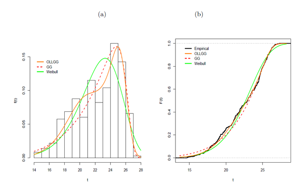
is really necessary. We provide the histogram of the data and the fitted density functions. Formal tests for the skewness parameter in the generated distribution can be based on LR statistics. The LR statistics for comparing the fitted models are listed in Table 7. We reject the null hypotheses in the two tests in favor of the wider distribution. The rejection is extremely highly significant and it gives clear evidence of the potential need for the shape parameter
when modeling real data. More information is provided by a visual comparison of the histogram of the data and the fitted density functions. The plots of the fitted OLLGG, GG and Weibull densities are displayed in Figure 9a. The estimated OLLGG density provides the closest fit to the histogram of the data.
Model |
|
|
|
|
|
AIC |
CAIC |
BIC |
OLLGG |
21.2911 |
13.0661 |
2.8755 |
0.2882 |
|
1752.1 |
1752.2 |
1767.7 |
|
(0.0012) |
(0.0234) |
(0.1095) |
(0.0127) |
|
|
|
|
KumGG |
25.3965 |
25.2759 |
12.8897 |
0.0243 |
2.3730 |
1780.6 |
1780.7 |
1800.1 |
|
(1.6147) |
(3.0850) |
(0.6885) |
(0.0079) |
(2.4887) |
|
|
|
EGG |
23.8850 |
22.9475 |
12.8766 |
0.0215 |
1 |
1777.6 |
1777.7 |
1793.2 |
|
(2.8175) |
(7.7331) |
(9.1805) |
(0.0019) |
|
|
|
|
GG |
26.1868 |
33.1789 |
0.1888 |
1 |
|
1777.6 |
1777.7 |
1788.3 |
|
(0.1877) |
(7.5737) |
(0.0514) |
(-) |
|
|
|
|
Weibull |
23.5808 |
9.4296 |
1 |
1 |
|
1796.4 |
1796.5 |
1804.2 |
|
(0.1376) |
(0.4038) |
(-) |
(-) |
|
|
|
|
|
|
|
|
|
|
|
|
|
BW |
25.0516 |
25.7636 |
0.2460 |
0.6159 |
|
1778.1 |
1778.3 |
1793.7 |
|
(1.3335) |
(8.2195) |
(0.0858) |
(0.4512) |
|
|
|
|
Table 6 MLEs of the model parameters for the temperature data and information criteria
Models |
Hypotheses |
Statistic w |
p-value |
OLLGG vs GG
OLLGG vs Weibull |
|
26.5
48.3 |
<0.0001
<0.0001 |
In order to assess if the model is appropriate, plots of the fitted OLLGG, GG and Weibull cumulative distributions and the empirical cdf are displayed in Figure 9b. They indicate that the OLLGG distribution gives a good fit to these data.
Under a Bayesian approach, we also fit the OLLGG model and some models described above. For each fitted model to these data, the Bayesian estimates of the model parameters and the DIC, EAIC and EBIC statistics are shown in the Tables 8 and 9, respectively. According to the three Bayesian information criteria, the OLLGG model stands out as the best one.
Survival data
Aids is a pathology that mobilizes its sufferers because of the implications for their interpersonal relationships and reproduction. Therapeutic advances have enabled seropositive women to bear children safely. In this respect, the pediatric immunology outpatient service and social service of Hospital das Cl´ınicas have a special program for care of newborns of seropositive mothers to provide orientation and support for antiretroviral therapy to allow these women and their babies to live as normally as possible. Here, we analyze a data set on the time to serum reversal of 148 children exposed to HIV by vertical transmission, born at Hospital das Cl´ınicas (associated with the Ribeirão Preto School of Medicine) from 1995 to 2001, where the mothers were not treated (Silva,30; Perdoná,31). Vertical HIV transmission can occur during gestation in around 35% of cases, during labor and birth itself in some 65% of cases, or during breast feeding, varying from 7% to 22% of cases. Serum reversal or serological reversal can occur in children of HIV-contaminated mothers. It is the process by which HIV antibodies disappear from the blood in an individual who tested positive for HIV infection. As the months pass, the maternal antibodies are eliminated and the child ceases to be HIV positive. The exposed newborns were monitored until definition of their serological condition, after administration of Zidovudin (AZT) in the first 24 hours and for the following 6 weeks. We assume that the lifetimes are independently distributed, and also independent from the censoring mechanism.

Figure 9 (a) Estimated densities of the OLLGG, GG and Weibull models for fibre data. (b) Estimated cumulative functions of the OLLGG, GG and Weibull models and the empirical cdf for temperature data.
Model |
|
|
|
|
|
OLLGG |
20.5189 (0.7529) |
12.6685 (1.2244) |
4.3121 (1.2345) |
0.2245 (0.0456) |
|
|
(18.8963, 21.8643) |
(10.2667, 14.8841) |
(2.0842, 6.8480) |
(0.1573, 0.3168) |
|
KumGG |
25.4831 (0.1970) |
25.7606 (0.2195) |
13.3406 (0.1878) |
0.0226 (0.00109) |
2.3779 (0.1234) |
|
(25.1727, 25.8274) |
(25.3986, 26.1771) |
(13.0556, 13.7286) |
(0.0205, 0.0247) |
(2.1607, 2.6765) |
EGG |
24.2333 (0.1250) |
23.9107 (0.3303) |
9.5727 (0.6326) |
0.0278 (0.0022) |
|
|
(23.9937, 24.4557) |
(23.3771, 24.4652) |
(8.6935, 10.9631) |
(0.0237, 0.0322) |
|
GG |
26.1305 (0.2334) |
32.4133 (7.9028) |
0.2104 (0.0669) |
|
|
|
(25.6783, 26.5446) |
(18.2675, 48.2415) |
(0.0981, 0.3381) |
|
|
Weibull |
23.5782 (0.1381) |
9.3741 (0.4078) |
|
|
|
|
(23.3033, 23.8465) |
(8.5262, 10.1351) |
|
|
|
Table 8 Posterior mean (standard deviation) and 95% Highest Posterior Density (HPD) interval of the model parameters
Model |
DIC |
EAIC |
EBIC |
OLLGG |
1746.344 |
1752.546 |
1768.146 |
KumGG |
1775.319 |
1783.009 |
1802.508 |
EGG |
1773.724 |
1779.722 |
1795.322 |
GG |
1774.657 |
1779.718 |
1791.418 |
Weibull |
1796.501 |
1798.483 |
1806.283 |
Table 9 Bayesian information criteria
Tables 10-12 list, respectively, the MLEs and their corresponding SEs in paren¬theses and posterior mean (standard deviation) and 95% highest posterior density (HPD) interval for the parameters and the values of the model selection statistics. These results indicate that the OLLGG model has the lowest AIC, BIC, CAIC, DIC, EAIC e EBIC values among those of all fitted models, and hence it could be chosen as the best model.
Note that the KumGG model is competitive with the model OLLGG. However, the model KumGG has two disadvantages:
It does not model bimodal data.
It has five parameters, i.e. is less parsimonious.
Model |
|
|
|
|
|
AIC |
BIC |
CAIC |
OLLGG |
352.0 |
46.9706 |
0.1043 |
0.4468 |
|
771.1 |
783.6 |
771.9 |
|
(1.0590) |
(1.4847) |
(0.0324) |
(0.0881) |
|
|
|
|
KumGG |
350.05 |
49.8303 |
0.2176 |
0.1282 |
0.3424 |
770.7 |
785.7 |
771.1 |
|
(1.5707) |
(5.8895) |
(0.0073) |
(0.0236) |
(0.0522) |
|
|
|
EGG |
350.45 |
22.2991 |
1.0741 |
0.1072 |
1 |
798.1 |
810.1 |
798.3 |
|
(2.4187) |
(0.0375) |
(0.0004) |
(0.0113) |
|
|
|
|
GG |
379.40 |
24.5312 |
0.0974 |
1 |
1 |
783.7 |
792.7 |
783.9 |
|
(8.8211) |
(10.3258) |
(0.0402) |
|
|
|
|
|
Weibull |
307.62 |
3.1132 |
1 |
1 |
1 |
808.0 |
814.0 |
808.1 |
|
(12.3523) |
(0.3250) |
|
|
|
|
|
|
|
|
|
a |
b |
|
|
|
|
BW |
349.99 |
6.3895 |
0.3944 |
0.9273 |
|
797.9 |
809.9 |
798.2 |
|
(23.0923) |
(0.7657) |
(0.0468) |
(0.3361) |
|
|
|
|
Table 10 MLEs of the model parameters for the serum reversal data, the corresponding SEs (given in parentheses) and the AIC, BIC and CAIC statistics
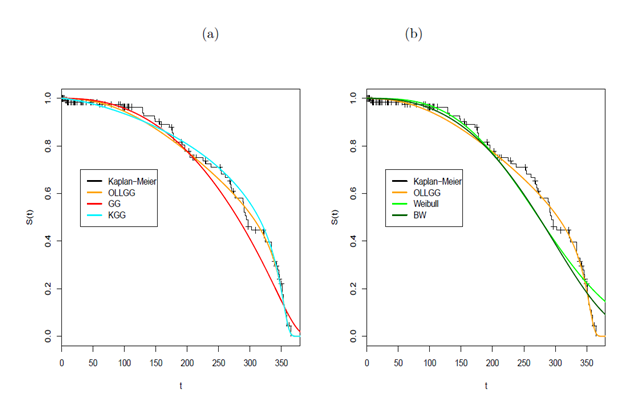
A comparison of the proposed distribution with some of its sub-models using LR statis¬tics is performed in Table 13. The figures in this table, specially the p-values, suggest that the OLLGG model yields a better fit to these data than the other three distributions. In order to assess if the model is appropriate, plots of the estimated survival functions of the KumGG, EGG, GG, Weibull and BW distributions and the empirical survival function are given in Figure 10. We conclude that the OLLGG distribution provides a good fit for these data.
Model |
|
|
|
|
|
OLLGG |
348.9 (11.5813) |
47.7542 (22.7428) |
0.1741 (0.1443) |
0.4342 (0.1619) |
|
|
(324.1, 366.5) |
(15.3289, 98.0374) |
(0.0230, 0.4910) |
(0.1331, 0.7222) |
|
KumGG |
351 (1.0623) |
42.8395 (1.4827) |
0.0114 (0.00383) |
3.0697 (0.5911) |
0.3601 (0.0550) |
|
(349.0, 353.1) |
(39.7113, 45.1984) |
(0.0058, 0.0191) |
(1.7862, 4.0205) |
(0.2678, 0.4790) |
EGG |
348.6 (0.8519) |
19.7657 (1.1290) |
4.3776 (1.0638) |
0.0309 (0.0097) |
|
|
(347.3, 350.4) |
(18.3590, 22.5768) |
(2.5525, 6.0764) |
(0.0177, 0.0505) |
|
GG |
376.3 (6.7347) |
44.2185 (16.2531) |
0.0652 (0.0341) |
|
|
|
(364.5, 389.9) |
(15.9226, 71.1764) |
(0.0279, 0.1302) |
|
|
Weibull |
307.5 (12.6278) |
3.0864 (0.3237) |
|
|
|
|
(283.7, 333.4) |
(2.4619, 3.7203) |
|
|
|
Table 11 Posterior means (Stantard Deviations) and 95% HPD intervals for the model parameters in the serum reversal data
Model |
DIC |
EAIC |
EBIC |
OLLGG |
752.017 |
775.385 |
787.3738 |
KumGG |
764.746 |
772.79 |
787.776 |
EGG |
781.475 |
788.53 |
800.519 |
GG |
776.599 |
783.425 |
792.417 |
Weibull |
807.984 |
809.989 |
815.983 |
Table 12 Bayesian information criterion
Model |
Hypotheses |
Statistic w |
p-value |
OLLGG vs GG
OLLGG vs Weibull |
|
13.0
40.3 |
0.00031
<0.0001 |
Table 13 LR statistics for the serum reversal data
Concluding remarks
The odd log-logistic generalized gamma (OLLGG) distribution provides a rather general and flexible framework for statistical analysis of positive data. It unifies some previously known distributions and yields a general overview of these distributions for theoretical studies. It also represents a rather flexible mechanism for fitting a wide spectrum of real world data sets. The OLLGG distribution is motivated by the wide use of the generalized gamma (GG) distribution in practice, and also for the fact that the generalization provides more flexibility to analyze skewed data. This extension provides a continuous cross over to other cases with different shapes (e.g. a particular combination of skewness and kurtosis). We derive an expansion for the density function as a linear combination of GG density functions. We obtain explicit expressions for the moments and moment generating function. The estimation of parameters is approached by the maximum likelihood method and a Bayesian approach, where the Gibbs algorithms along with metropolis steps are used to obtain the posterior summaries of interest for survival data with right censoring. Two applications of the OLLGG distribution to real data show that it could provide a better fit than other statistical models frequently used in lifetime data analysis.

Figure 10 Estimated survival function by fitting the OLLGG distribution and some other models and the empirical survival for the serum reversal data. (a) OLLGG vs KGG and GG. (b) OLLGG vs BW and Weibull.
Acknowledgments
Conflicts of interest
References
- Gleaton JU, Lynch JD. On the distribution of the breaking strain of a bundle of brittle elastic fibers. Advances in Applied Probability. 2006;36(1):98–115.
- Braga AS, Cordeiro GM, Ortega EMM, et al. The odd log-logistic normal distribution: Theory and applications in analysis of experiments. Journal of Statistical Theory and Practice. 2016;10(2):311–335.
- da Cruz JN, Ortega EMM, Cordeiro GM. The log-odd log-logistic Weibull re-gression model: Modelling, estimation, influence diagnostics and residual analysis. Journal of Statistical Computation and Simulatio. 2016;86(8):1516–1538.
- Cordeiro GM, Ortega EMM, Silva GO. The exponentiated generalized gamma distribution with application to lifetime data. Journal of Statistical Computation and Simulation. 2011;81(7):827–842.
- Pascoa MAR, Ortega EMM, Cordeiro GM. The Kumaraswamy generalized gamma distribution with application in survival analysis. Statistical Methodology. 2011;8(5):411–433.
- Ortega EMM, Cordeiro GM, Pascoa MAR. The generalized gamma geometric distribution. Journal of Statistical Theory and Applications. 2011;10(3):433–454.
- Cordeiro GM, Castellares F, Montenegro LC, de Castro M. The beta generalized gamma distribution. Statistics. 2013;47(4):888–900.
- Lucena SEF, Silva AH, Cordeiro GM. The transmuted generalized gamma distribution: Properties and application. Journal of Data Science. 2015;13(1):409–420.
- Silva RB, Bourguignon M, Cordeiro GM. A new compounding family of dis- tributions: The generalized gamma power series distributions. Journal of Computational and Applied Mathematics. 2016;303(C):119–139.
- http://www.tandfonline.com/doi/abs/10.1081/STA-120003130
- Stacy EW. A generalization of the gamma distribution. Annals of Mathematical Statistics. 1962;33(3):1187–1192.
- Stacy EW, Mihram GA. Parameter estimation for a generalized gamma distri- bution. Technometrics. 1965;7(3):349–358.
- Lawless JF. Statistical Models and Methods for Lifetime Data. 2nd ed. New York, USA;2003.
- Mudholkar GS, Srivastava DK. Exponentiated Weibull family for analyzing bathtub failure-rate data. IEEE Transactions on Reliability. 1993;42(2):299–302.
- Mudholkar GS, Srivastava DK, Freimer M. The exponentiated Weibull family: A reanalysis of the bus-motor-failure data. Technometrics. 1995;37(4):436–445.
- Nadarajah S. The exponentiated Gumbel distribution with climate application. Environmetrics. 2005;17(1):13–23.
- Shirke DT, Kakade CS. On exponentiated lognormal distribution. International Journal of Agricultural and Statistical Sciences. 2006;2:319–326.
- Nadarajah S, Gupta AK. The exponentiated gamma distribution with application to drought data. Calcutta Statistical Association Bulletin. 2007;59:29–54.
- Nadarajah S, Kotz S. The exponetiated type distributions. Acta Applicandae Mathematicae. 2006;92(2):97–111.
- Gradshteyn and Ryzhik's Table of Integrals, Series, and Products. 6th edn. Alan Jeffrey and Daniel Zwillinger; 2000.
- Nadarajah S. Generalized gamma variables with drought application. Journal of the Korean Statistical Society. 2008;37(1):37–45.
- Murphy JA. Handbook of hypergeometric integrals-theory, application, tables, computer programs, by Harold Exton, Ellis Horwood Limited, Chichester, 1978. No. of pages: 316, price £15. International Journal for Numerical Methods in Engineering. 1979;14(1):1–155.
- Aarts RM. Lauricella functions. From MathWorld, A Wolfram Web Resource, created by Eric W Weisstein. 2000.
- http://www.emeraldinsight.com/doi/pdfplus/10.1108/10610420610679593
- Spiegelhalter DJ, Best NG, Carlin BP, et al. Bayesian measures of model complexity and fit. Journal of the Royal Statistical Society Series. 2002;B64(4):583–639.
- Brooks SP, Jim Smith, Aki Vehtari, et al. Discussion on the paper by Spiegelhalter, Best, Carlin, and van der Linde. Journal of the Royal Statistical Society. Series B: Statistical Methodology. 2002;64(4):616–639.
- Carlim BP, Louis TA. Bayes and empirical bayes methods for data analysis. 2nd edn. In: Chapman and Hall. Boca Raton, Florida, USA. 2001;85(503): 381-383.
- Cordeiro GM, Alizadeh M, Tahir MH, et al. The beta odd log-logistic generalized family of distributions. Hacettepe Journal of Mathematics and Statistics. 2016;45: 1–28.
- Famoye F, Lee C, Olumolade O. The beta-Weibull distribution. Journal of Statistical Theory and Applications. 2005;4:121–136.
- Silva ANF. Estudo evolutivo das criancas expostas ao HIV enotificadas pelo nucleo de vigilancia epidemiologica do HCFMRP-USP. M.Sc. Thesis. University of Sao Paulo, Brazil. 2004.
- Perdona GSC. Modelos de riscos aplicadosa analise de sobrevivencia. Doctoral Thesis, Institute of Computer Science and Mathematics, University of Sao Paulo, Brasil. 2006.

©2017 Prataviera,, et al. This is an open access article distributed under the terms of the,
which
permits unrestricted use, distribution, and build upon your work non-commercially.


