Research Article Volume 7 Issue 5
Smoothing parameter estimation for first order discrete time infinite impulse response filters
Livio Fenga
Italian National Institute of Statistics, Italy
Correspondence: Livio Fenga, Italian National Institute of Statistics, Italy, Tel 3906 4673 3222
Received: August 27, 2018 | Published: October 22, 2018
Citation: Fenga L. Smoothing parameter estimation for first order discrete time infinite impulse response filters. Biom Biostat Int J. 2018;7(5):483-489. DOI: 10.15406/bbij.2018.07.00250
Download PDF
Abstrat
Discrete time Infinite Impulse Response low-pass filters are widely used in many fields such as engineering, physics and economics. Once applied to a given time series, they have the ability to pass low frequencies and attenuate high frequencies. As a result, the data are expected to be less noisy. A properly filtered signal, is generally more informative with positive repercussions involving qualitative aspects – e.g. visual inspection and interpretation – as well as quantitative ones, such as its digital processing and mathematical modelling. In order to effectively disentangle signal and noise, the filter smoothing constant, which controls the degree of smoothness in First Order Discrete Time Infinite Impulse Response Filters, has to be carefully selected. The proposed method conditions the estimation of the smoothing parameter to a modified version of the information criterion of the type Hannan - Quinn which in turns is built using the Estimated Log Likelihood Function of a model of the class SARIMA (Seasonal Auto Regressive Moving Average). Theoretical evidences as well as an empirical study conducted on a particularly noisy time series will be presented.
Keywords: big data, discrete time infinite impulse response filters, denoising, hannan quinn information criterion, sarima models, time series
Introduction
Among the many denoising methods and techniques successfully employed for univariate time series – e.g. based on regression,1 Kalman filter,2,3 decomposition,4 wavelet5,6 and non-linear method7– those based on algorithms of the type Infinite Impulse Response (IIR) exponential filters have been massively used, given their satisfactory performances (see, for example,8 and, more recently9). Such methods are useful for their ability to maximize the amount of relevant information that can be extracted from “real life” time series. In fact, regardless the scientific field time dependent data are collected for (e.g. engineering, economics, physics, environmental), they can never be error–free. In spite of all of the efforts and precautions one might take in order to provide clean data – e.g. robust data acquisition methods, reliable routine checks, sophisticated procedures for error correction, fail safe data storage and data communication lines – reality is way too complex for such procedures to be completely reliable.
Noise, in fact, is simply an ubiquitous entity able to affect virtually all the stages a given analysis of a time series can be broken into, showing uncountable expressions that can be only partially controlled, never fully removed nor exactly pinpointed. Many are the fields where noise reduction methods are employed: data mining, satellite data, radio communications, radar, sonar and automatic speech recognition, are just a few of them. Often, the treatment of noisy data is critical, as in the case of bio–medical signals, tracking systems for defense purposes or economics, where the trend or the seasonal patterns of vital economic variables can be obscured or distorted by noise components. However, the type of time series likely to be easily affected by noise – as well as by sudden or unpredictable high frequency variations – can be found in the economic and social fields. A telling example, is the great deal of data generated by web–based services (e.g. Google or Twitter), which are commonly and publicly available, in many instances free of charge. However, statistical estimation procedures based on this type of data can embody many sources of uncertainty and instability. They are related, for example, to technical (computer alphabetization) or psychological (e.g. emotional driven spikes and other form of data perturbations) reasons. Even when data are collected and validated by Official Organisms (e.g. national and super-national statistical offices or central banks), strong psychological components can play a significant role in determining erratic and/or noisy behaviors. This is the case, for instance, of the Economic Sentiment Indicators – provided by many National Institute of Statistics – which are purposely designed to capture the amount of optimism (pessimism) towards the future behavior of a set of economic variables. Being these data able to reflect, at least to some extent, the future decision making strategies of a population of reference, they can show dangerous instabilities and irregularities. In other words, when an opinion is in the process to form or change then many analysts are mostly interested in its future developments; however, this is usually the points in time where the data show complex structures, which are usually hard to capture.
The need to conduct more precise model–based investigations under noisy data structures has been the motivating factor of the proposed method. As it will be seen, it delivers interesting performances and is reasonably fast, the latter characteristic making the proposed method a viable option with high dimensional data sets, e.g. of the type big data. It is also risk–free, i.e. when there are no filtering–related benefit – according to a suitable objective function – the method is designed to simply leave the data unfiltered (the
–smoothing parameter is set to
). The paper proceeds as follows: in Section 2 the problem is defined along with the statistical model assumed for the underlying data generating mechanism, whereas in Section 3 the employed low–pass filter is illustrated, with a special focus on its calibration issues. The method is explained in Section 4 and the step-by-step implementation of the algorithm is given in paragraph 4.3. Finally, an empirical experiment, conducted on a time series provided by the search engine Google and recovered in the repository called Google Trends (for Italy the address is https://trends.google.it/trends/?geo=IT), is presented in section 5.
Statement of the problem
Throughout the paper, the time series (also defined as signal) of interest is intended to be a real–valued, uniformly sampled, sequence of data points of length
, denoted as:
(1)
Each datum
, being observed with an error, say
, is called
in contrast with the “pure’, noise–free, unobservable one
. Therefore, the formal set up is of the type
It is worth stressing that the theoretical framework we are dealing with, does not envision
as being the standard
–mean constant variance
idiosincratic component. In fact,
can also embody all the unpredictable components arising when “real–life” signals come into play and which, in general, are able to generate unwanted phenomena, like sudden outburst of energy (outliers) and noise. As a consequence, at least two detrimental effects are embedded in the signal and can affect its statistical properties: accuracy reduction and generation of heavy noisy components. The former relates to the addiction (subtraction) of significant quantities to (from)
, so that we have
, while the latter is a subtler, but nonetheless dangerous, disturbing phenomenon. It arises, for example, when in a survey some statistical units are not longer available and must be replaced by “similar” ones. When such a corrupted information set is applied as an input to a mathematical model for any purposes, e.g. simulation or prediction, the related outcomes are likely to be affected.
The data generating process
The observed signal is supposed to be a realization of a statistical model of the class
(Seasonal Auto Regressive Integrated Moving Average), which is a generalization of the
(Auto Regressive Integrated Moving Average) class proposed by George et.,10 have been introduced to model complex dynamics i.e. of the type stochastic seasonal. It can be expressed as:10,11
where
denotes the backward shift operator,
and
denote the non – seasonal and seasonal difference operator respectively and:
;
;
;
;
;
with
,
,
,
, respectively, the non seasonal autoregressive and moving average parameters and the seasonal autoregressive and moving average parameters. Finally
is a
-mean and finite variance white noise. The model can be estimate when the stationary and invertibility conditions are meet for both the autoregressive and moving average polynomials respectively, that is
=0 and
=0 have their root lying outside the unit circle. Generally, this model is abbreviated as
. When the process is stationary and no seasonal patterns are detected, the model collapses to a pure
model. The explanation of the ARIMA theory is outside the scope of this paper, therefore the interested reader is referred to Makridakis8 and Stock.12
Under Gaussianity, the SARIMA parameter vector
(2)
can be estimated via Conditional
(Maximum Likelihood Estimation) method, which:
- In the version employed to run the empirical experiment (Section 5), uses the joint probability density function for
, i.e.
-
and
- Maximizes the function given by
with
being recursively estimated using
(3)
Equation (3) holds by equating the first
observations to 0, i.e.
and setting the first
innovations to 0:
.
The employed filter
By the Central Limit Theorem, by “properly” averaging sub-sequences of a noisy signal, a better approximation of the “true” ones is obtained as a result.13 Consistently, one strategy for noise control relies on a filter of the type discrete time Infinite Impulse Reponse.14 This class of filters is a powerful tool for handling noise in many fields: in15 its performances has been compared with many other methods on environmental data (other than simulated ones) whereas its application for standard control-chart procedures is documented in Layth et al.,16 and Stuart Hunter.17 Its usefulness for interactive systems and information extraction for complex turbulent flows has been discussed respectively in Casiez18 and Adrien Cahuzac,19 whereas the effectiveness of smoothing–driven approaches in economic time series forecasting is documented in the excellent book from Hyndman et al.,20 and in Codrut.21
IIR filters envision the level of the stochastic process (1) at a given time
, say
to be dependent to the present and past observations according to
Using the lag operator
, such that
, (4) can be re-expressed as
(4)
and rewritten as
(5)
From (5) it is evident that
is a weighted average of
(current datum) and the previous level
, whose weight sequence is determined by the smoothing parameter
. Finally, (4) can be expressed, by skipping the lag operator, in a recurrence form as
(6)
or in a error correction form, i.e. determined by the equation
, as follows:
The form (6) is the one used in the sequel. Here, the first term represents the contribution added by each and every datum updating our time series whereas the second one accounts for the inertia from the previous observations. Therefore, the amount of noise left in the signal as well as the system lag (the responsiveness of the system output to changes in the input) are both proportional to
.
It is worth emphasizing that the order of a low–pass filter reflects the amount of strength it uses to attenuate a predetermined frequency band. First order filters of the type (4) reduce the signal amplitude by half for each frequency doubling while higher order filters amplify this effect proportionally with their order. For the purpose pursued here, the order 1 appeared to be appropriate since the filter is:
[(a)]
- “Only” required to denoise (e.g. no forecasting purposes are pursued);
- Easier to tune;
- More interpretable.
However, properly tuning the constant parameter is not a trivial task nor something that – at least in general – can be left to subjective judgment. In fact, a too high
can leave significant amount of idiosincratic components in the signal while too low values determine the speed at which the older data are dampened to be too slow (over smoothing).
The smoothing constant and the objective function
As already pointed out, the smoothing parameter (also called smoothing factor or smoothing constant), controls the amount of past information contributing to the formation of the present signal level. Formally, a point in time distant
lags influences the level of the signal at time
by an amount given by
. Even though the proposed method is designed to provide an estimate of
, it might be interesting to investigate the frequency property of the filter, in order to obtain meaningful information from the selected
. The related cut–off frequency can be derived15,22 by
–transorming (6), i.e.
which can be regarded as the digital version of the analog filter (6). By defining
as the sampling period and equating
to the frequency
, i.e.
;
, the power spectra of
and
, respectively called
and
are related to each other through
(7)
By equating the first term in (7) to
, the cut–off frequency at which the amplitude is reduced by a factor of 2, say
, is found, i.e.
and therefore
The above approximation is possible being in practice
, for the temporal integration to be possible.
The Hannan–Quinn information criterion
As it will be outlined in the sequel, the smoothing constant is the minimiser of a penalized Log-Likelihood function, estimated on a model of the class SARIMA applied to both the original and filtered time series
. The objective function chosen belongs to the class of the information criterion, i.e. the Hannan-Quinncriterion.23 This order selector has been constructed from the law of iterated algorithm and shows a penalty function growing at a very slow rate, as the samples size increases. It is defined as follows:
being
the vector of the estimated SARIMA parameters of (??) whereas
is the Likelihood function.
By estimating the log–likelihood function
with
and writing the penalty term as
k
, the Hannan Quinn information criterion can be written as
where also the subscript
, stands for “observed”.
The standard identification procedure for the selection of the best SARIMA model order under this information criterion, follows the general rule as the other Information Criteria and is denoted as Minimum Information Criterion Estimation (
). In essence, it is based on the minimization of the information criterion itself. Here, the model
minimizing the HQ criterion, is the winning one, that is:
(8)
with
as defined in (2).
The method
The proposed method can be regarded as an optimal averaging procedure under a penalized log–likelihood function. “Properly” averaging a signal as a noise reduction method is consistent to the principle that, if repeated measures are conducted many times on a given signal, part will tend to accumulate but the noise will be irregular and tend to cancel itself. This result is connected to the fact that the mean standard deviation of N measurements is smaller by a factor of N than the standard deviation of a single measurement. Practically, if one compute the average of “many” samples of a noisy signal the noise–induced random fluctuations tend to die out and the signal is therefore stronger.
In more details, when one records the signal
(1)
times (the sampling rate) over a predefined time interval, say
, being
, he can compute
averages each of length
. Two critical points arise at this time, i.e. how many data points should be averaged and in which manner. The latter question has been already answered (Section 3) whereas the former – which is strictly related with the smoothing parameter
– controls the number of observations of
to be averaged (and to what extent), so that the noise which randomly fluctuate with equal probability above or below the “true” level
tends to cancel out while the signal builds up.
The
parameter is chosen as the minimizer of (8) once a “great” number of candidates
is tried. Therefore, (8) is modified as
(9)
being
.
What presented in (9) is a slightly modified version of the Hannan Quinn criterion, called here
(which will be justified below), whose minimum value delivers the optimal smoothing parameter
.
From the last equation, it is clear that both the optimal model and the optimal
are simultaneously estimated. However, while the
parameters’ estimation is conducted on the filtered versions
of the observed signal, the variance parameter is estimated using the observed data
. Such an operation is possible assuming
and serves the purpose to “force” the filtered output to be “not too far” from the observed signal
. In practice, the Information Criterion selects an “optimal” model – built on a
–filtered version of the data (which therefore are used to build the ML estimations of the
parameters) whose goodness of fit is computed with respect the observed (noisy) signal
. In other words, mHQ criterion has a stronger penalty than the standard one. Such an additional weight (the penalty associated with the residual variance computed on
) is proportional to
and serves the purpose to prevent the H-Q criterion from choosing
values that can lead to over smoothing. In fact, the greater the value of
the greater the distance between
and
and therefore the greater the absolute values of the difference
. When no benefit can be obtained by applying the filter, we have
therefore
and
coincide and
, i.e. the best SARIMA model is built on
and its order selection follows the MICE rule according to equation (8). On the contrary, when a benefit from filtering is detected – i.e.
– therefore the best model is the one built on the filtered time series according to a
value (
) at which the information criterion (9) is minimized and its order selection follows the MICE rule. Again, such a conclusion is justified as the error term is “average out” by the filter. At this point, we have two different SARIMA models fitting
and
and generating two error vectors. Recalling (3), and consistently with the notation so far used, it will be
(10)
and
found in a similar way, replacing the superscript identified by the letter
with the Greek letter
.
Moreover, by virtue of Granger theorem,24 it is always possible for an estimated SARIMA model order to depart from the “true” one when the input is affected by white noise components. In such a case, the CSS estimates resulting from the function
can be regarded as converging to the pseudo–true value of the parameters’ vector and therefore the order detected by means of the
– which employs the function
for the estimation of the parameters – criterion will be closer to the “true” model order.
Signal improvement assessment
At this point, it is clear that for
the lower bound in the gain delivered by the procedure is attained (i.e. no gain and
). In this section, a simple way for assessing the performances of the filter (if delivered) is presented. At this point it might be worthwhile emphasizing that the method presented in this paper is not designed to improve the forecasting performance of SARIMA models. In fact, the observations coming from the future, under an unchanged data generation mechanism, will be affected, in average, by the same noise components affecting the previous observations. However, projecting the filtered observations into the future is a useful exercise for at least two reasons: i) to verify that the forecasting performances delivered by the two SARIMA models are “not too far” from each other (meaning that the
is a “bona fide” version of the original one; ii) in many cases, improvements in the forecasting performances have been observed. This can be explained by the fact that the order selection and estimation procedures tend to work better under less noisy signals.
With that said, the signal-to-noise ratio (SNR) has been used as an indicator of the quality of the filtered signal. It is defined as the ratio of the power of the signal (the meaningful information) to the power of the noise (the unwanted portion of the signal). In its “pure” form it is
,
being the average power. In the framework at hand, both the power levels are estimated by their respective variances
, being the error terms obtained using (10). Practically, by comparing
with
, one is able to assess how much of the unwanted components has been removed under
The algorithm
In what follows, the method is presented in the form of a step–by–step algorithm. In particular, steps 2-6 are conducted on the training set whereas the remaining 7–8 use the test set.
- The time series under investigation is split in two sets: training and test;
- A grid of tentative smoothing constant
is built;
- A SARIMA model is estimated on the original time series
using the H–Q criterion;
-
SARIMA models are estimated on
filtered time series
;
- If
stop and use the unfiltered time series otherwise proceed;
- The
smoothing constant associated with the winner model (according to the modified H–Q criterion mHQ) is then chosen;
- Horizon
forecast mean square errors are computed for both the filtered and unfiltered series;
- Both the statistics are compared for consistency.
Clearly, if one is not interested in forecast comparison – e.g. to speed up the computations and have faster outcomes – then steps 1, 7 and 8 can be skipped.
Empirical experiment
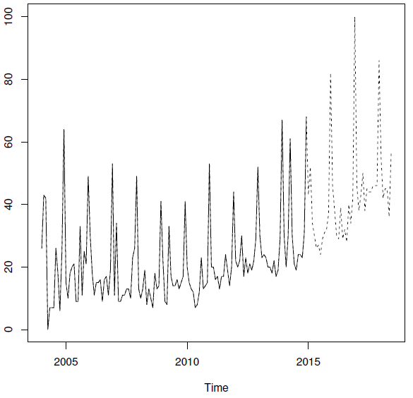
The experiment presented in this paragraph is aimed at showing the capabilities of the proposed method. A time series – collected by the popular search engine Google and recovered in an “ad hoc” repository called Google Trends – will be employed. It refers to the relative number of Italian Internet users which inputted the keyword “caviar” (caviale, in Italian) into the search engine Google, between January 2004 and June 2018. The data have been download on June 6th 2018 (h 03:29 PM GMT). Time series length is 174, split in training set – ending in December 2014 (132 data) – and test set (42 data), ending in June 2018. The last datum has been purposely left in the data set, for it is an even more unstable one (in fact, it is supported only by a small portion of the month of reference). A visual inspection of the series, depicted in Figure 1, shows many irregularities, a pronounced, non stationary seasonality as well as a non stationary trend. Eteroschedasticity is also an issue. Such a behavior might be considered typical for a luxury good especially when observed, as in the present case, for a long period of time.

Figure 1 Relative number of the keyword “caviar” searched by the Italian Internet users. Training set (continuous line) and test set (dashed line).
The whiteness of the residuals has been tested using a test of the type “Portmanteau’, i.e. the Ljung-Box test,25 which is designed to account for the sum of the autocorrelations (denoted by the Greek letter
) until a predetermined, arbitrary lag
, i.e.
Publication
Here
is, for significance level
, the critical region for rejection of the hypothesis of randomness under the
distribution.
The estimated SARIMA order in the case of
is
with an HQ criterion of 4.97. In the case of
, the estimated SARIMA order is
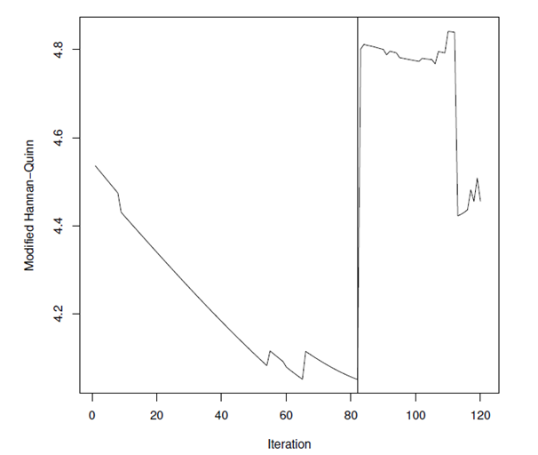
, for a modified HQ criterion equal to 4.05. Therefore, the filter is applied. The effects of its application are presented in Figure 2, where a more regular signal can be noticed. Such an impression is confirmed by looking at the SNRs, which is equal to 6.88 and 7.06 respectively for the unfiltered and filtered time series. The optimal smoothing constant
, has been obtained at iteration number 82 (see Figure 3), using a grid of 121
values (equally spaced from 0.400 to 1; incremental step= 0.005). The residuals (computed in both the cases on the original time series) pass the ‘Portmanteau’ test (computed for the lags 1–24) only in the case of
(p value
), whereas for the raw signal we have p value
. Such a conclusion is consistent with the patterns shown by the empirical autocorrelation functions (see Figure 4) for
(graph a) and
(graph b). In the same graph, the residual density distributions for
(graph c) and
(graph d) confirm a better behavior when the proposed method is applied. Finally, in Figure 5, the prediction performances obtained using
appears to be slightly better until lag 8.
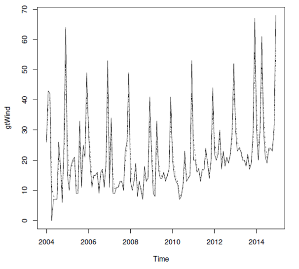
Figure 2 Unfiltered (continuous line) and filtered (dashed line) time series.

Figure 3 Values of the modified Hanna–Quinn information criterion for each iteration (attempted
value). The vertical line shows the iteration number at which the minimum mHQ value is found.
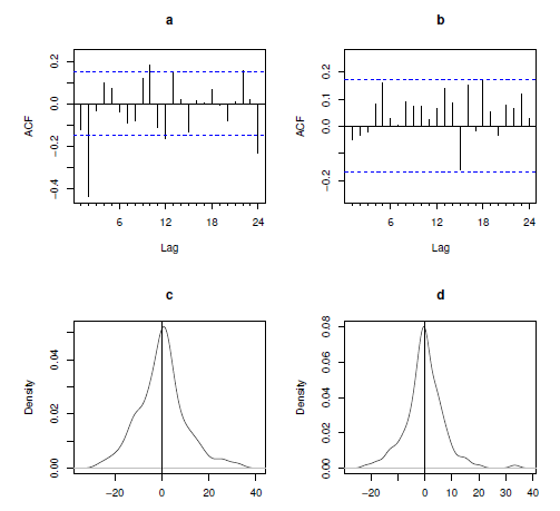
Figure 4 Autocorrelation functions for
(graph a),
(graph b) and residual density for
(graph c) and
(graph d).
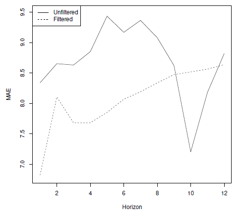
Figure 5 Mean Absolute Error of the predictions obtained from the two SARIMA models applied on the raw time series (continuous line) and the filtered time series (dashed line). Time horizon 1–12.
Conclusion
One effective way to reduce noise components affecting our time series is to use a First Order Discrete Time Infinite Impulse Response Filter. As it is well known, its filtering performances are critically dependent on the smoothing constant, which therefore has to be carefully fine–tuned. The method proposed in this paper provides the practitioner with a useful – and reasonably fast – tool to filter out such unwanted components. However, that the objective function used – based on the Hannan Quinn information criterion – has given good results, does not imply that is the best possible one. For example, with small data set it could be worth considering different information criteria, specifically designed for such a case, e.g. the second-order AIC.26 Finally, different stochastic models can be always considered, according to the underlying data generating process. For instance, whenever the time series shows memory characteristics of the type long range, the proposed procedure can be associated to a suitable model (e.g. of the class Autorgressive Fractional Integrated Moving Average).
Acknowledgements
Conflict of interest
Author declares that there is no conflict of interest.
References
- Richard T O'Connell, Anne B Koehler. Forecasting, time series, and regression: An applied approach, volume 4. USA: South–Western Pub; 2005.
- Ruey S Tsay. Analysis of Financial time series. Volume 543. USA: John Wiley & Sons; 2005.
- Harold Wayne Sorenson. Kalman ltering: theory and application. IEEE. 1985.
- Phillip G Gould, Anne B Koehler, J Keith Ord, et al. Forecasting time series with multiple seasonal patterns. European Journal of Operational Research. 2008;191(1):207–222.
- David L Donoho. De–noising by soft–thresholding. IEEE transactions on information theory. 1995;41(3):613–627.
- Albert Cohen, Ingrid Daubechies, Bjorn Jawerth, et al. Multiresolution analysis, wavelets and fast algorithms on an interval. Comptes Rendus de l Académie des Sciences. 1993;316(5):417–421.
- Holger Kantz, Thomas Schreiber. Nonlinear time series analysis, volume 7. USA: Cambridge university press; 2004.
- S Makridakis. Forecasting: Methods and applications. 1998.
- Torsten kohler, Dirk Lorenz. A comparison of denoising methods for one dimensional time series. Bremen: Germany, University of Bremen; 2005.
- George EP Box, Gwilym M Jenkins, Gregory C Reinsel, et al. Time series analysis: forecasting and control. USA: John Wiley & Sons; 2015.
- Peter J Brockwell, Richard A Davis. Time series: theory and methods. Springer Science & Business Media. 2013.
- JH Stock, MW Watson. Introduction to econometrics. Boston: Addison–wesley; 2003.
- MJ Evanich, AO Newberry, LD Partridge. Some limitations on the removal of periodic noise by averaging. Journal of Applied Physiology. 33(4):536–541;1972.
- CC Holt. Forecasting trends and seasonals by exponentially weighted averages. carnegie institute of technology. Technical report, Pittsburgh ONR memorandum. 1957.
- Adrien Cahuzac, Jerome Boudet, Pierre Borgnat, et al. Smoothing algorithms for mean–ow extraction in large–eddy simulation of complex turbulent ows. Physics of uids. 2010;22(12):125104.
- Layth C Alwan, Harry V Roberts. Time series modelling for statistical process control. Statistical Process Control in Automated Manufacturing. 1988;15:45–65.
- J Stuart Hunter. The exponentially weighted moving average. Journal of quality technology. 1986;18(4):203–210.
- Gery Casiez, Nicolas Roussel, Daniel Vogel. 1 euro Filter: a simple speed–based low–pass Filter for noisy input in interactive systems. In: Proceedings of the SIGCHI Conference on Human Factors in Computing Systems. ACM. 2012;2527–2530.
- Adrien Cahuzac, Jerome Boudet, Pierre Borgnat, et al. Smoothing algorithms for mean–ow extraction in large–eddy simulation of complex turbulent ows. Physics of uids. 2010;22(12):125104.
- Rob Hyndman, Anne B Koehler, J Keith Ord, et al. Forecasting with exponential smoothing: the state space approach. Springer Science & Business Media. 2008.
- Fat Codrut, A Maria, Dezsi Eva, et al. Exchange–rates forecasting: Exponential smoothing techniques and arima models. Annals of Faculty of Economics. 2011;1(1):499–508.
- Athanasios Papoulis. Signal analysis. volume 191. New York: McGraw–Hill; 1977.
- Edward J Hannan, Barry G Quinn. The determination of the order of an autoregression. Journal of the Royal Statistical Society. Series B (Methodological). 1979; 190–195.
- Clive WJ Granger. Essays in econometrics: collected papers of Clive WJ Granger. Volume 32. USA: Cambridge University Press; 2001.
- Greta M Ljung, George EP Box. On a measure of lack of t in time series models. Biometrika. 1978;65(2):297–303.
- Kenneth P Burnham, David R Anderson. Model selection and multimodel infer–ence: a practical information–theoretic approach. Springer Science & Business Media. 2003.

©2018 Fenga. This is an open access article distributed under the terms of the,
which
permits unrestricted use, distribution, and build upon your work non-commercially.


