eISSN: 2378-315X


Research Article Volume 5 Issue 5
Rutgers University, USA
Correspondence: Duo Zhou, Rutgers University, 9 Stuart Ln E, Princeton Junction, NJ 08550, Tel 703-888-9296
Received: March 10, 2017 | Published: April 13, 2017
Citation: Zhou D. Prognostic factors and predictions of survival data using cox ph models and random survival forest approaches. Biom Biostat Int J. 2017;5(5):165-181. DOI: 10.15406/bbij.2017.05.00142
Survival outcome has been one of major endpoints for clinical trials; it gives information on the probability of time-to-event of interest. Recently, there has been increasing demands for survival analysis tools, especially for high dimensional survival data. Most of the classical statistical approaches including nonparametric, semi-parametric and complete parametric models, have limitations. Typical nonparametric approaches, such as the logrank (or Cox-Mantel) test, do not have stringent models assumptions, but can only deal with a limited number of categorical predictors. Typical semi-parametric approaches, such as Cox proportional hazard (PH) model, have stringent model assumptions, such as linearity, interactions and proportionality; and they can only deal a limited number of predictors. Complete parametric models, such as accelerated failure time models, are similar to semi-parametric models except that they make further assumptions about the baseline hazard function.
In this paper, non-parametric random survival forest approaches were introduced with many advantages over typical nonparametric, semi-parametric or parametric approaches. They have very no model assumptions and can deal with many more predictors than typical survival models. Two Cox PH models were evaluated and the model performances were compared with the random survival forest models based on a simulation study. Additionally, the random survival forest approaches were further studied based on a real world case study, which included more predictors then a typical Cox PH model can handle.
Keywords: cox proportional hazard model, nonlinear, proportionality, random forest, survival, prediction errors, AUCs, time-dependent, time-varying
Survival data arise from many fields, such as medicine, biology, public health, epidemiology, etc. Although the analysis approaches discussed in this paper should be general and applicable to all of these disciplines, the research interest focused on biological, medical or clinical applications.
Most if not all survival analysis approaches are focused on survival (or time-to-event) outcomes, which are usually associated with serious disease conditions, such as death, heart failures and recurrence of cancers. Typically, survival outcome includes one binary variable for occurrence(s) of the event(s) of interest and at least one continuous variable for the time of the occurrence(s) or the censoring time (2 time variables may be needed for the intervals within which the event occurs). The outcome is referred to as time-to-event, which has been one of the major endpoints for clinical studies.
To best utilize such data, different approaches are developed to exploit the complete information about the occurrence of the event and the timing of the event. Recently, there has been increasing demand for survival analysis tools, especially for high dimensional survival data. Most of the classical statistical approaches including nonparametric, semi-parametric and complete parametric models have limitations. Typical nonparametric approaches, such as the logrank (or Cox-Mantel) test, do not have stringent model assumptions, but can only deal with a limited number of categorical predictors. Typical semi-parametric approaches, such as Cox PH models, however rely on more stringent model assumptions, such as linearity, interactions and proportionality; and they work only if the number of predictors is fewer than the number of events. Complete parametric models, such as accelerated failure time models, are similar to semi-parametric models except that they make further assumptions about the baseline hazard function.
In this paper, we employed a systematic process to assess the assumptions for typical Cox models. For linearity assumption, appropriate nonlinear functional forms were recommended if necessary; for interaction effects, appropriate interactions were suggested if detected; for proportionality assumptions, appropriate extension model was attempted to resolve non-proportionality.
In summary, two typical Cox PH models were intended, Cox PH linear model without consideration of nonlinearity and Cox PH model with RCS transformations for adjustment of nonlinearity; two nonparametric random survival forest approaches, a logrank based random survival forest1(LR-RSF) developed by Mogensen and Ishwaran (2012) and a conditional-inference based random survival forest2,3(CINF-RSF) suggested by Hothorn et al. (2006) were also implemented. All of these intended approaches were compared in terms of prognostic factor detections and prediction performance.
These approaches, including the Cox PH linear model and Cox PH model with RCS transformation, LR-RSF and CINF-RSF models, were assessed via a simulation study; the performance of these models was compared in terms of prediction errors and prediction AUCs. The LR-RSF and CINF-RSF models were further evaluated based on a real world case study, where typical Cox PH models did not work due to too many predictors and too little events.
For both studies, the original data were randomly partitioned into training and testing sets with 3:1 ratio; the training set was used for model selections and cross validations; the test set was used for assessment of the prediction performance
Simulation studies with time-varying treatment effect
A total of 2000 subjects were simulated using R4 Software; 7 factors included age, sex, race, systolic blood pressure (SBP), diastolic blood pressure (DBP), body mass index (BMI) and treatment were generated from computer programs. SBP and DBP were generated from two normal distribution with correlated coefficients of 0.9; and they were weakly correlated with BMI (SBP and BMI: =0.3; SBP and BMI: = 0.2). Once all factors were generated, time-to-events were simulated from the factors following a pre-specified exponential model. A time-varying treatment was also generated: subjects were randomized to active and placebo treatment at baseline. However, subject randomized to placebo at baseline were allowed to switch to active treatment after the 1 year follow-up. The actual reasons for treatment switch could be very subjective, but for this study, the treatment switch was randomly generated for the placebo randomized subjects. Further simulation details are not presented in this paper.
Real world case study
A breast cancer data with 5 clinical factors and 70 gene signatures obtained from the Netherlands Cancer Institute was used to evaluate metastasis-free survival, which will be called NKI705 data onward. The data included a total of 144 independent lymph-node-positive breast cancer subjects, followed for 17 months; 48 subjects experienced a metastasis event.
For this study, the number of factors were more than the number of event ; typical Cox models did not work, only LR-RSF and CINF-RSF models were implemented.
Analysis method
In general, the following 5 functions are used to describe survival data: (1) survival function, (2) density probability function, (3) cumulative probability function, (4) hazard function and (5) cumulative hazard function. A basic problem in survival analysis is to estimate one or more of these five functions from the collected survival data and to draw inferences about the survival patterns in the population.4 The formulations of the 5 functions do not involve any assumptions; hence they are still considered as nonparametric and can be applied across all survival models.
Cox PH linear model: Typical Cox PH linear model are commonly expressed as,
(1)
where all factors or composite factors are included in their 1st order linear form and potential 2nd order interaction terms between the original factors (or composite factors) are also considered; this model is referred to as Cox PH linear model. For this model, if composite factors are derived, they should be included to replace the original factors they are clustered from. The best model are achieved following a backward step-down selection procedure. This model was implemented with R/rms7 package from Harrell (2014).
Cox PH model with RCS transformation: A Cox PH model with RCs transformation is implemented to account for nonlinearity; potential interactions between the actual functional forms of the factors are also considered. For this model, nonlinear continuous factors are transformed using restricted cubic spline (RCS) function. If interactions are detected, the terms should include the RCS transformations of the factors involved in the interactions. For time varying treatment effect, the subject who switched treatment were considered as having two different observations, each with a different treatment and a corresponding time interval; Andersen-Gill extension of the Cox PH model are implemented for the adjustment. The Cox PH models with RCS transformations can be formulated similar to Equation 1, except that some covariates may have nonlinear forms of the original factors. This model were implemented with R/rms7 package.
Random survival forest (RSF) models: Two forms of random survival forest (RSF) were implemented. One was based on the logrank test; this approach is referred to as logrank-based RSF model (LR-RSF). Another form was built on conditional inference based logrank test; where multiple significance tests are computed at each start of the algorithm based on permutation test; this approach is referred to as conditional-inference-based (CINF-RSF) model. Both of the RSF mode are based on logrank scores; of which, the test statistics can be obtained as
(2)
where the superscripts and refer to the two offsprings of the parent node from the tree splitting; is the number of distinct event times and refers to the time .
The LR-RSF model was implemented with R/random Survival SRC8-10 package developed by Ishwaran and Kogalur (2013) and CINF-RSF model was implemented with R/party2,11,12 package developed by Hothorn et al. (2006).
Evaluation of model performance: The model performance is evaluated using Brier scores13 as proposed by Gerds et al. (2006) and time-dependent AUCs. The Brier Score at time, , is defined as:
Brier Score at (3)
Where is the observed survival status at time , which is is the predicted survival probability at time , is the total number of subjects. The prediction error, , is used to estimate the prediction performance at time . The integrated Brier score is obtained by averaging the total Brier scores for interval , which can be expressed as , where different event times.
AUC is another assessment for model performance, which is estimated using c-index, as recommended by Harrell (2012); c-index is the probability of concordant pairs of predicted and observed cases among all pairs of responses. Specifically, if the predicted survival time (or probability) is larger for the subject who (actually) lived longer, the predictions for that pair are said to be concordant with the (actual) outcomes. Similar to prediction errors, time-dependent AUCs can be estimated.
The performance statistics and corresponding 95 percentile intervals (95% PCIs) can be estimated with the mean and the 95 percentiles from bootstrapped samples of the test set.
Results of the simulation study
Summary statistics of the simulation study: Summary of demographics for the simulated study is not presented. Summary of subject survival status at 1-year post baseline and treatment switching after 1-year post baseline is presented in Table 1. For this simulation study, 106 (10.6%) subjects from active treatment arm had events prior to 1 year and 163 (16.3%) subjects from the placebo (SOC) arm had events prior to 1 year. Of the 891 subjects randomized to active treatment who survived 1 year, none of the subjects switched to placebo; of the 840 subjects randomized to placebo and survived 1 year, 201 (23.9%) switched to the active treatment, and the rest of the 639 subjects stayed in the placebo arm until censored or failed.
Enrollment Randomization |
|||
Status or Treatment |
Active |
Placebo (N=1003) |
|
Survival at Year -1 Status |
Event Free |
891 (89.4%) |
840 (83.7%) |
After Year-1 |
Active Treatment |
891 |
840 |
Table 1 Survival Status at 1-Year and Treatment Switching After 1-Year Post Baseline
Preparations for analysis: As mentioned earlier, subjects who were randomized to placebo at baseline were allowed to switched to active treatment after 1-year post baseline; according to the intent-to-treat (ITT) principal, these subjects were assumed to be treated with placebo as intended and assumed to follow the hazard from the placebo arm even after the switching; neglecting the benefit from the active treatment due to treatment switching led to violation of proportionality, the scaled Schoenfeld residual was significantly correlated with time ; the downwarding slope of the scaled Schoenfeld residual plot as shown in Figure 1 also confirmed non-proportionality.
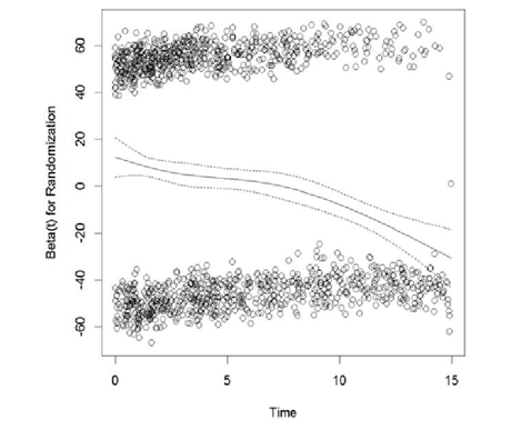
Apparently, treatment was changing over time for these subjects; to adjust for time-varying treatment effect, each of each subjects were assumed to have multiple observations corresponding to the different treatments overt time, Andersen-Gill extension of Cox PH model was implemented. The scaled Schoenfeld residuals from the adjusted model are plotted in Figure 2. The scaled Schoenfeld residual plot is almost parallel to the x-axis; the proportionality test was no longer significant ( ).
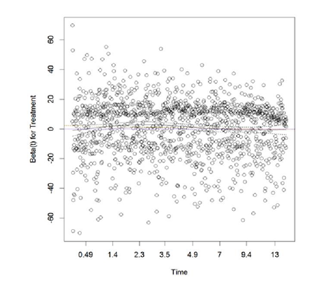
Thus, non-proportionality was resolved for treatment.
Additionally, SBP and DBP were highly correlated, from which a composite factor MAP was derived; thus the factor MAP would be used to replace SBP and DBP for survival models.
Linearity, interactions and proportionality: For Cox PH linear model, linearity was assumed for all factors; for Cox model with RCS transformations, the functional forms were visually examined with the Martingale residual plot, which was obtained from a tentative model with the original factors. Figure 3 displays the Martingale residuals vs. each of the continuous factors stratified by the actual Treatment. The observational-level residuals are presented in the top half of the figure and the subject-level residuals are presented in the bottom. From the subject-level residual plot, 3 inflection points were observed for Age and MAP, 1 inflection point was observed for BMI; to be more conservative, 5-knot RCS transformation for Age and MAP, 3-knot RCS transformation for BMI was considered in the initial model with RCS transformations.
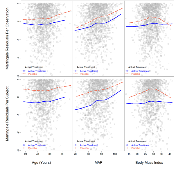
Additionally, the smoothed lowess curves of Age were parallel between treatments, which suggested no interaction between Age and treatment. For MAP, the lowess curves for different treatments had different slopes, thus interaction was suggested. For BMI, the placebo group had shown slight quadratic pattern, but pretty much straight for the Active treatment; however the overall pattern did not suggest interaction. For further investigation, a model with all interactions involving treatment was intended. Results are presented in Table 2; significant P-value was a strong evidence of interaction. Overall, Age, BMI and Sex had no interactions with Treatment, but MAP and Race might interact with Treatment.
d.f. |
P-value |
||
Treatment |
74.82 |
6 |
<.0001 |
All Interactions |
9.07 |
5 |
0.1065 |
Age |
3.11 |
2 |
0.2109 |
With Treatment |
0.03 |
1 |
0.8553 |
MAP |
54.28 |
2 |
<.0001 |
With Treatment |
5.54 |
1 |
0.0186 |
BMI |
1.23 |
2 |
0.5408 |
With Treatment |
0.41 |
1 |
0.5204 |
Sex |
31.64 |
2 |
<.0001 |
With Treatment |
1.32 |
1 |
0.2511 |
Race |
25.56 |
2 |
<.0001 |
With Treatment |
2.51 |
1 |
0.113 |
Total Interaction |
9.07 |
5 |
0.1065 |
TOTAL |
175.73 |
11 |
<.0001 |
Table 2 Wald Test on Interactions between Treatment and All Other Factors – Simulation Study
Similarly, interactions involving Sex and interactions involving Race were also examined separately. Interaction between Sex and Race was suggested; interactions between Sex and MAP, between Race and BMI were questionable. For the initial survival model, all potential interactions were included; the initial Cox PH model with RCS transformations is formulated as
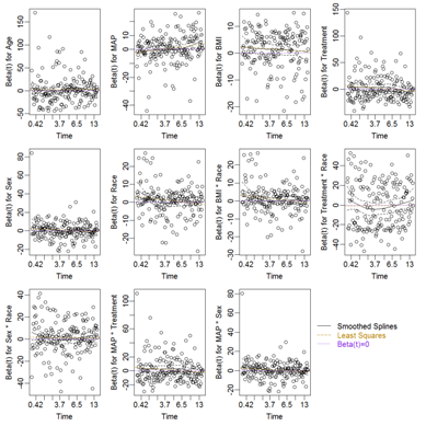
Proportionality assumptions were further examined using a Cox PH model with RCS transformation as presented in Equation 4; the Scaled Schoenfeld residual plots are presented in Figure 4 and the results of the Wald tests for proportionality are presented in Table 3. Non-proportionality was not found for any of the predictors.
Factors |
P |
|||
Age |
- |
-0.0112 |
0.16 |
0.687 |
MAP |
- |
-0.0012 |
0 |
0.963 |
BMI |
0.001 |
0 |
0.971 |
|
Treatment |
- |
-0.0363 |
1.85 |
0.174 |
Sex |
- |
-0.019 |
0.57 |
0.448 |
Race |
-0.0191 |
0.5 |
0.48 |
|
BMI:Race |
- |
-0.0206 |
0.58 |
0.446 |
Treatment:Race |
- |
0.0032 |
0.01 |
0.906 |
Sex:Race |
- |
0.0094 |
0.12 |
0.726 |
MAP:Treatment |
- |
-0.0328 |
1.51 |
0.22 |
MAP:Sex |
- |
-0.0194 |
0.6 |
0.438 |
GLOBAL |
- |
NA |
9.35 |
0.589 |
Table 3 Proportionality Test on Each of the Predictor in the Cox PH model with RCS Transformation – Simulation Study
Analysis (Model selection)
Cox PH linear regression: The Cox PH linear model was implemented including all factors in their original scale and the 2nd order interactions. Models were selected using backward step-down procedure with AIC as the selection rule. Once the best model was achieved, the regression coefficients, the corresponding standard errors and P-values were estimated from the final Cox PH linear model; results are presented in Table 4.
|
Coef |
SE |
Z |
Pr(>|Z|) |
Age |
0.004 |
0.0023 |
1.86 |
0.0628 |
{Male} |
-0.301 |
0.0557 |
-5.41 |
<.0001 |
Race {Black} |
0.328 |
0.1275 |
2.57 |
0.0102 |
{Hispanic} |
0.029 |
0.1312 |
0.22 |
0.8241 |
{White} |
0.017 |
0.1202 |
0.14 |
0.8894 |
MAP |
0.046 |
0.0074 |
6.18 |
<.0001 |
{Active Treatment} |
1.429 |
0.8407 |
1.7 |
0.0892 |
MAP:{Active Treatment} |
-0.022 |
0.0096 |
-2.25 |
0.0242 |
Table 4 Regression Coefficients of the Selected Model for Conventional Cox Regression with Linear Forms of All Factors – Simulation Study
The log hazard and hazard ratios from the final model are summarized in Table 5. For continuous factor, the low and high are the minimum and maximum of the factor; the difference was the difference between the maximum and the minimum; the effect, the lower and upper 95% CI were the log hazard (/ hazard ratios), the lower and upper bounds of the 95% CIs with respect to unit change in the factor.
Low |
High |
Diff. |
Effect Lower 95% CI |
Upper 95% CI |
||
Age |
42.67 |
57.96 |
15.29 |
0.067 |
-0.0034 |
0.1365 |
Hazard Ratio |
42.67 |
57.96 |
15.29 |
1.069 |
0.9966 |
1.1463 |
MAP |
82.85 |
90.69 |
7.84 |
0.388 |
0.2427 |
0.5341 |
Hazard Ratio |
82.85 |
90.69 |
7.84 |
1.475 |
1.2747 |
1.706 |
Sex - Male:Female |
1 |
2 |
-0.298 |
-0.4081 |
-0.1889 |
|
Hazard Ratio |
1 |
2 |
0.742 |
0.6649 |
0.8278 |
|
Race - Black:Asian |
1 |
2 |
0.33 |
0.0801 |
0.5801 |
|
Hazard Ratio |
1 |
2 |
1.391 |
1.0834 |
1.7863 |
|
Race - Hispanic:Asian |
1 |
3 |
0.035 |
-0.2228 |
0.2926 |
|
Hazard Ratio |
1 |
3 |
1.036 |
0.8003 |
1.34 |
|
Race - White:Asian |
1 |
4 |
0.02 |
-0.2157 |
0.2561 |
|
Hazard Ratio |
1 |
4 |
1.02 |
0.806 |
1.2919 |
|
Treatment - Active:Placebo |
1 |
2 |
-0.452 |
-0.5645 |
-0.3403 |
|
Hazard Ratio |
1 |
2 |
0.636 |
0.5686 |
0.7116 |
|
Table 5 Summary of the Regression Coefficients of the Best Selected Model for Conventional Cox Regression with Linear Forms of All Factors – Simulation Study
In this table, the interaction effects were not presented separately from the individual factors, instead they were summarized by different level of the factors involved in the interactions: the hazard ratio between Active Treatment and Placebo was obtained based on the median MAP.
The performance for the final Cox PH linear model were measured with prediction errors and time-dependent AUCs, which were assessed based on the test set; results are summarized in Table 6. The prediction errors were calculated based on Equation 3; the AUC was the area under the ROC curve; a value of 0.5 corresponded to the probability of a random guess and a value of 1 corresponded to 100% accuracy; smaller prediction error or large AUCS suggested better predictions. The prediction errors and time-dependent AUCs and the corresponding 95% PCIs are displayed in Figure 5. The survival probability of future events and median survival time for each subject can be predicted; results are not presented.
|
Prediction Error |
AUC |
Yrs |
(95% PCI) |
(95% PCI) |
1 |
0.112 (0.093, 0.133) |
0.683 (0.619, 0.746) |
2 |
0.167 (0.149, 0.185) |
0.644 (0.597, 0.692) |
3 |
0.202 (0.187, 0.216) |
0.632 (0.590, 0.675) |
4 |
0.218 (0.207, 0.228) |
0.631 (0.596, 0.671) |
5 |
0.232 (0.222, 0.242) |
0.622 (0.587, 0.659) |
6 |
0.235 (0.224, 0.247) |
0.621 (0.589, 0.654) |
7 |
0.233 (0.219, 0.248) |
0.619 (0.589, 0.653) |
8 |
0.229 (0.212, 0.247) |
0.618 (0.588, 0.649) |
9 |
0.221 (0.201, 0.243) |
0.617 (0.588, 0.648) |
10 |
0.210 (0.184, 0.233) |
0.617 (0.588, 0.648) |
11 |
0.201 (0.172, 0.228) |
0.617 (0.588, 0.649) |
12 |
0.192 (0.161, 0.222) |
0.618 (0.589, 0.648) |
13 |
0.188 (0.152, 0.222) |
0.617 (0.588, 0.647) |
14 |
0.179 (0.141, 0.217) |
0.616 (0.588, 0.647) |
Table 6 Prediction performance of the best selected model for Cox PH linear model –simulation study
Cox PH model with RCS transformation: The initial Cox PH model with RCS transformation was intended with Equation 4. Similar to what was done for Cox PH linear model, the above model was backward selected following a step-down procedure using AIC as the selection rule. The final Cox PH model with RCS transformation obtained from the procedure is summarized in Table 7. The final reduced model can be formulated as
Coef |
S.E. |
Z |
P(>|Z|) |
|
Sex=Male |
6.243 |
3.8531 |
1.62 |
0.1052 |
Race=Black |
0.326 |
0.1293 |
2.52 |
0.0116 |
Race=Hispanic |
0.045 |
0.1328 |
0.34 |
0.7326 |
Race=White |
0.028 |
0.1214 |
0.23 |
0.8169 |
Treatment=Active |
-0.475 |
0.0574 |
-8.28 |
<.0001 |
BMI |
0.026 |
0.0151 |
1.73 |
0.0844 |
BMI' |
-0.043 |
0.0177 |
-2.43 |
0.0149 |
MAP |
0.063 |
0.0417 |
1.5 |
0.1337 |
MAP' |
-0.14 |
0.1816 |
-0.77 |
0.4403 |
MAP'' |
0.99 |
1.0592 |
0.93 |
0.3498 |
MAP''' |
-1.824 |
1.7453 |
-1.05 |
0.296 |
Sex=Male : MAP |
-0.084 |
0.0487 |
-1.72 |
0.0859 |
Sex=Male : MAP' |
0.544 |
0.2209 |
2.46 |
0.0137 |
Sex=Male : MAP'' |
-4.148 |
1.3237 |
-3.13 |
0.0017 |
Sex=Male : MAP''' |
7.952 |
2.2253 |
3.57 |
0.0004 |
Table 7 Regression Coefficients of the Best Model for Multivariate Cox Regression with RCS Transformations – Simulation Study
The log hazards and hazard ratios from the selected Cox model with RCS transformations are presented in Table 8. For continuous factors, the effect, the corresponding lower and upper bound of the 95% CI with respect to unit change are presented.
Low |
High Diff. |
Effect |
Lower 0.95 |
Upper 0.95 |
||
BMI |
25.95 |
31.48 |
5.52 |
-0.0359 |
-0.1106 |
0.0387 |
Hazard Ratio |
25.95 |
31.48 |
5.52 |
0.9647 |
0.8953 |
1.0395 |
MAP |
82.85 |
90.69 |
7.84 |
0.3373 |
0.1054 |
0.5692 |
Hazard Ratio |
82.85 |
90.69 |
7.84 |
1.4012 |
1.1112 |
1.7669 |
Sex - Male:Female |
1 |
2 |
-0.046 |
-0.2621 |
0.1701 |
|
Hazard Ratio |
1 |
2 |
0.955 |
0.7694 |
1.1854 |
|
Race - Black:Asian |
1 |
2 |
0.3262 |
0.0728 |
0.5797 |
|
Hazard Ratio |
1 |
2 |
1.3857 |
1.0755 |
1.7854 |
|
Race - Hispanic:Asian |
1 |
3 |
0.0454 |
-0.2148 |
0.3056 |
|
Hazard Ratio |
1 |
3 |
1.0464 |
0.8067 |
1.3574 |
|
Race - White:Asian |
1 |
4 |
0.0281 |
-0.2098 |
0.2661 |
|
Hazard Ratio |
1 |
4 |
1.0285 |
0.8107 |
1.3048 |
|
Treatment - Active:Placebo |
1 |
2 |
-0.4754 |
-0.5879 |
-0.3629 |
|
Hazard Ratio |
1 |
2 |
0.6216 |
0.5555 |
0.6956 |
|
Table 8 Summary of Log Hazards and Hazard Ratios of All Factors from the Selected Model for Multivariate Cox Regression with RCS Transformations – Simulation Study
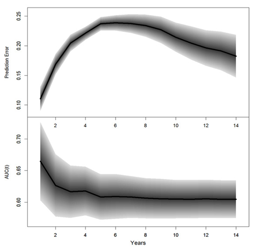
The prediction performance of the final Cox model with RCS transformations was measured with prediction errors and time-dependent AUCS again based on the test set; the prediction errors, the time-dependent AUC and the corresponding 95% PCIs are summarized in Table 9; the corresponding plots are displayed in Figure 6. With the selected model, the predicted log-hazards, survival and median survival time were obtained for each subject in the test; the results are not presented in this paper.
|
Prediction Error |
Time-Dependent AUCs |
Yrs |
(95% PCI) |
(95% PCI) |
1 |
0.112 (0.091, 0.132) |
0.665 (0.601, 0.724) |
2 |
0.169 (0.151, 0.186) |
0.627 (0.578, 0.676) |
3 |
0.205 (0.191, 0.2187) |
0.617 (0.575, 0.658) |
4 |
0.221 (0.210, 0.233) |
0.618 (0.578, 0.655) |
5 |
0.237 (0.225, 0.248) |
0.608 (0.572, 0.644) |
6 |
0.239 (0.225, 0.251) |
0.609 (0.574, 0.646) |
7 |
0.238 (0.222, 0.253) |
0.608 (0.575, 0.642) |
8 |
0.234 (0.215, 0.252) |
0.606 (0.574, 0.638) |
9 |
0.227 (0.205, 0.249) |
0.605 (0.574, 0.637) |
10 |
0.214 (0.190, 0.239) |
0.605 (0.574, 0.635) |
11 |
0.205 (0.177, 0.234) |
0.605 (0.574, 0.635) |
12 |
0.196 (0.168, 0.228) |
0.605 (0.575, 0.635) |
13 |
0.191 (0.160, 0.225) |
0.605 (0.575, 0.635) |
14 |
0.182 (0.147, 0.219) |
0.605 (0.575, 0.634) |
Table 9 Prediction Performance of the Selected, Cox PH model with RCS Transformations – Simulation Study
Logrank based random survival forest (LR-RSF): As mentioned earlier, LR-RSF could not handle multiple observations per subject from the time- varying treatment effect; thus subjects who switched from placebo to active treatment were considered as 2 independent subjects, each with a different treatment for different durations. Nonetheless, LR-RSF is nonparametric without any assumptions, thus nonlinearity or non-proportionality was not concerned.
As previously mentioned, MAP was a composite factor derived from SBP and DBP, they were highly correlated. To keep consistent with the Cox PH models, the initial RSF models were intended with Age, MAP, BMI, Sex, Race and Treatment. Table 10 presents the VIMP of all factors excluding SBP and DBP. The plots of out-of-Bag (OOB) error rate and VIMP with SBP and DBP excluded are presented in Figure 7; significant change was not observed.
VIMP |
Relative VIMP |
|
MAP |
0.0081 |
1 |
Sex |
0.008 |
0.9887 |
Race |
0.0041 |
0.5026 |
BMI |
0.0021 |
0.2646 |
Age |
0.0004 |
0.053 |
Treatment |
0.0004 |
0.0501 |
Table 10 VIMP from LR-RSF with SBP
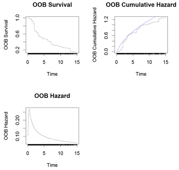
The cross validated LR- RSF model was then used for predictions of future events and assessment of prediction performance. The OOB survival, cumulative hazard and hazard for a subset of 3 subjects are presented in Figure 8 and the overall OOB survival probability, Brier scores and mortality are presented in Figure 9. The predicted mortality and survival probability for each subject in the test set were obtained; results are not presented in this paper. The model performance were assessed again with the test set, the results will be presented later in Table 11 and Error! Reference source not found. for comparison with CINF-RSF model.
Prediction Errors |
Time-Dependent AUCs |
||||||
Yrs |
LR-RSF (95% PCI) |
CINF-RSF (95% PCI) |
Cox |
LR-RSF (95% PCI) |
CINF-RSF (95% PCI) |
Cox |
|
1 |
0.111 (0.091, 0.133) |
0.112 (0.093, 0.134) |
0.112 |
0.652 (0.584, 0.718) |
0.653 |
(0.589, 0.721) |
0.683 |
2 |
0.167 (0.150, 0.192) |
0.168 (0.154, 0.194) |
0.167 |
0.638 (0.590, 0.687) |
0.613 |
(0.563, 0.655) |
0.644 |
3 |
0.199 (0.184, 0.218) |
0.202 (0.191, 0.219) |
0.202 |
0.645 (0.603, 0.686) |
0.624 |
(0.585, 0.662) |
0.632 |
4 |
0.218 (0.205, 0.233) |
0.218 (0.213, 0.232) |
0.218 |
0.636 (0.600, 0.673) |
0.619 |
(0.587, 0.656) |
0.631 |
5 |
0.243 (0.229, 0.255) |
0.233 (0.230, 0.250) |
0.232 |
0.612 (0.580, 0.649) |
0.607 |
(0.576, 0.639) |
0.622 |
6 |
0.246 (0.231, 0.261) |
0.236 (0.226, 0.252) |
0.235 |
0.607 (0.574, 0.642) |
0.611 |
(0.582, 0.643) |
0.621 |
7 |
0.249 (0.231, 0.265) |
0.234 (0.224, 0.256) |
0.233 |
0.602 (0.570, 0.636) |
0.605 |
(0.576, 0.637) |
0.619 |
8 |
0.243 (0.224, 0.261) |
0.229 (0.220, 0.257) |
0.229 |
0.602 (0.568, 0.633) |
0.596 |
(0.569, 0.630) |
0.618 |
9 |
0.230 (0.208, 0.253) |
0.222 (0.207, 0.251) |
0.221 |
0.598 (0.568, 0.631) |
0.596 |
(0.570, 0.629) |
0.617 |
10 |
0.216 (0.189, 0.243) |
0.209 (0.191, 0.243) |
0.21 |
0.593 (0.564, 0.626) |
0.599 |
(0.572, 0.630) |
0.617 |
11 |
0.202 (0.175, 0.230) |
0.200 (0.178, 0.234) |
0.201 |
0.597 (0.568, 0.631) |
0.6 |
(0.572, 0.632) |
0.617 |
12 |
0.193 (0.168, 0.220) |
0.192 (0.167, 0.225) |
0.192 |
0.591 (0.564, 0.627) |
0.594 |
(0.567, 0.623) |
0.618 |
13 |
0.185 (0.152, 0.213) |
0.188 (0.159, 0.225) |
0.188 |
0.582 (0.554, 0.614) |
0.584 |
(0.558, 0.614) |
0.617 |
14 |
0.172 (0.142, 0.205) |
0.180 (0.150, 0.219) |
0.179 |
0.571 (0.544, 0.603) |
0.576 |
(0.553 0.602) |
0.616 |
Table 11 Prediction Errors and AUCs for LR-RSF, CINF-RSF and Conventional Cox PH Linear Model – Simulation Study
Conditional inference based random survival forest (CINF-RSF): Another nonparametric CINF-RSF model was also cross validated with the training set. A CINF-RSF tree is presented in Figure 10; survival plots are displayed in the terminal node.
LR-RSF vs. CINF-RSF: For detecting prognostic factors, both managed to pick up the most important factors, although slight difference was observed between the two RSF models. The prediction performance of the two approaches were further assessed and compared in terms of prediction errors and time-dependent AUCs.
The prediction errors and time-dependent AUCS for LR-RSF and CINF-RSF and the corresponding 95% PCIs are summarized in Table 11 and the prediction errors and AUCs from the reduced Cox PH linear model are also presented as a reference; the corresponding plots are displayed in Figure 12. The black solid curve and the gray shaded area is the performance and the corresponding 95% PCIs for CINF- RSF; the red dashed curve with light pink shaded area is the performance and the 95% PCIs for LR-RSF; the blue dotted curves is the performance from the Cox PH linear model.
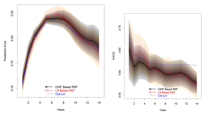
In terms of prediction errors, the Cox PH linear model performed slightly better than the two RSF models; the two RSF models were similar to each other within the first 5 years; LR-RSF was worse than the CINF-RSF model between 5 and 10 years and at the tail (beyond year-10), LR-RSF performed slightly better than CINF-RSF. In terms of time-dependent AUCs, the Cox PH linear model still performed the best; the two RSF models had the maximum difference within the first 5 years, after which the two models were similar.
Comparisons of all intended models: In summary, the Cox PH linear model had the best performance of all intended models; while the 2 RSF models were much easier to implement and the prediction performance was satisfactory. Both RSF models can deal with more predictors than typical Cox PH models can handle; they are nonparametric without stringent assumptions, so they were much easier to implement. Between the 2 RSF models, LR-RSF is more favorable if covariates are not highly correlated; while CINF-RSF performs better for highly correlated data. There is one pitfall for LR-RSF model, it could not account for multiple observations per subject, which could lead to the slightly worse performance.
For cross comparisons, the prediction errors and time-dependent AUCs for the 4 intended models are displayed again in Figure 13 and Figure 14, respectively. Of the 4 models, the Cox PH linear model and CINF-RSF model had almost equivalent prediction errors and LR-RSF model had the worst prediction errors in general. Surprisingly, the Cox model with RCS transformation had slightly worse prediction errors than the Cox PH linear model, probably because the former picked up BMI instead of Age. In terms of time-dependent AUCs, the Cox PH linear model performed the best overall; the AUC of the LR-RSF inclined a little between year 2-5, otherwise, it had similar performance to the CINF-RSF; the AUC of the Cox PH model with RCS transformation was similar to the CINF-RSF within the first half of the study, then it became the second best at the tail (slightly worse than the Cox PH linear model). Additionally, both Cox PH models provided unbiased parameter estimates which were easy to interpret; while the RSF models did not provide parameter estimates and were relative more difficult to interpret.
However, considering the nonparametric nature, the prediction performance of the two RSF models was satisfactory and both models picked up the right set of factors without making stringent assumptions.
Results of real world case study
Summary of the NKI70 data: For NKI70 data, only the 5 clinical factors and 2 of the 70 gene signatures are summarized in Table 12. Contingency tables for categorical factors are presented in the top half of the table and continuous factors, including Age and 2 of the 70 gene signatures are summarized in the bottom. Full summary of all gene signatures will not be presented but can be provided upon request. One clinical factor, grade of tumor, had 3 categories; 2 dummy variables were created for the relative difference between categories. Thus, a total of 76 factors should be considered.
Factors |
Statistics (N=144) |
Survival: Metastasis |
48 (33%) |
Diameter of Tumor |
|
≤ 2 cm |
73 (51%) |
> 2 cm |
71 (49%) |
Number of affected lymph nodes |
|
1-3 |
106 (74%) |
≥ 4 |
38 (26%) |
Estrogen receptor status |
|
Negative |
27 (19%) |
Factors |
Statistics (N=144) |
Positive |
117 (81%) |
Grade of tumor |
|
Poorly Differentiated |
48 (33%) |
Intermediate |
55 (38%) |
Well Differentiated |
41 (28%) |
Factors (71) |
n/nmiss |
Mean ± SD |
Median |
Quartiles |
Ranges |
Age |
144/0 |
44.31 ± 5.34 |
45 |
41, 49 |
16 – 53 |
TSPYL5 |
144/0 |
-0.109 ± 0.33 |
-0.089 |
-0.331, 0.117 |
-1.08 – 0.6018 |
DIAPH3 |
144/0 |
-0.033 ± 0.24 |
-0.022 |
-0.179, 0.241 |
-0.679, 0.618 |
- |
- |
- |
- |
- |
- |
C20OR46 |
144/0 |
-0.086 ± 0.25 |
-0.133 |
-0.256, 0.020 |
-0.451 – 0.992 |
Table 12 Brief Summary of the NKI70 Data
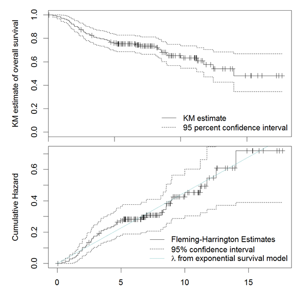
Data preparation: The Kaplan-Meier (KM) estimates of the survival probability and the Fleming-Harrington estimates of the log cumulative hazard are displayed in Figure 15; the green dotted line superimposed on top of the cumulative hazard was the hazard assuming exponential survival models; where little change was observed in the slope of cumulative hazard over time. Thus, it was reasonable to consider Cox model. Figure 16 displays the correlation map of all factors; blue color indicated a positive correlation and red color indicated a negative correlation. The intensity of the color indicated the severity of collinearity. Apparently, several of the gene-signatures were highly correlated.
For this case study, typical Cox models did not work for too many predictors with too few events; only the LR-RSF and CINF-RSF models were intended. Again, the two RSF models were nonparametric without stringent assumptions.
Logrank Based Random Survival Forest (RSF): For this case study, LR-RSF was first implemented. Table 13 presents the variable importance (VIMP) of a subset of factors; the gene signature, GPR180, was the least important with VIMP of -0.0027; 3 genes with the least absolute VIMP (VIMP = 0) were Grade. Intermediate, Contig40831.RC and PECI.1; the factors with VIMP ≥ 0.0027, which is the absolute value of the least VIMP, should be potentially important. Figure 17 displays the CV error and VIMP for all factors; the LR-RSF model was stabilized at 25 trees, although the model still exhibited some variations which was common for bootstrap aggregations. For VIMP plot, factors were ordered from the least to the most VIMP; the factors with negative VIMP were colored in red and positive VIMP were colored in blue.
Factors |
VIMP |
Relative VIMP |
Factors |
VIMP |
Relative VIMP |
ZNF533 |
0.0236 |
1 |
Diam.GT2 |
0.0028 |
0.1167 |
PRC1 |
0.0108 |
0.4598 |
DTL |
0.0027 |
0.1165 |
QSCN6L1 |
0.007 |
0.296 |
- |
- |
- |
RFC4 |
0.0066 |
0.2778 |
Grade. Intermediate |
0 |
0.0015 |
CDCA7 |
0.0046 |
0.197 |
Contig40831.RC |
0 |
-0.0012 |
IGFBP5 |
0.0046 |
0.1934 |
PECI.1 |
0 |
-0.002 |
SLC2A3 |
0.0034 |
0.1434 |
- |
- |
- |
N.GE4 |
0.0028 |
0.1178 |
GPR180 |
-0.0027 |
-0.1137 |
Table 13 VIMP from LR-RSF – NKI70 Data
The OOB survival, Brier scores and mortality for all subjects in the training set were obtained from cross validation (CV); results are plotted in Figure 18. The cross validated LR-RSF model was used for predictions based on the test set; the predicted mortality and survival were obtained, but the results are not presented in this paper. The prediction errors and time-dependent AUCs were assessed again based on the test set; results will be presented later in Table 14 for comparison with CINF-RSF model.
Prediction Errors |
Time-Dependent AUCs |
|||||||
Months |
LR-RSF (95% PCI) |
CINF-RSF (95% PCI) |
LR-RSF (95% PCI) |
CINF-RSF (95% PCI) |
||||
1 |
0.0536 |
(0.0005, 0.1343) |
0.0518 |
(0.0009, 0.1291) |
0.7131 |
(0.5532, 1.0000) |
0.7648 |
(0.6146, 1.0000) |
2 |
0.0953 |
(0.0314, 0.1769) |
0.0915 |
(0.0292, 0.1723) |
0.7054 |
(0.5667, 0.8258) |
0.7559 |
(0.6239, 0.8699) |
3 |
0.1631 |
(0.0802, 0.2453) |
0.1554 |
(0.0733, 0.2394) |
0.7025 |
(0.5469, 0.8278) |
0.7564 |
(0.6235, 0.8676) |
4 |
0.1786 |
(0.1087, 0.2545) |
0.1739 |
(0.1005, 0.2509) |
0.6966 |
(0.5000, 0.8290) |
0.7572 |
(0.6270, 0.8665) |
5 |
0.2064 |
(0.1300, 0.2756) |
0.213 |
(0.1325, 0.2925) |
0.6729 |
(0.5000, 0.8253) |
0.7544 |
(0.6199, 0.8673) |
6 |
0.2019 |
(0.1293, 0.2684) |
0.2083 |
(0.1310, 0.2859) |
0.6589 |
(0.5000, 0.8156) |
0.7527 |
(0.6126, 0.8707) |
7 |
0.2165 |
(0.1512, 0.2892) |
0.2238 |
(0.1503, 0.2990) |
0.6746 |
(0.5000, 0.8158) |
0.7533 |
(0.6100, 0.8663) |
8 |
0.2165 |
(0.1512, 0.2892) |
0.2238 |
(0.1503, 0.2990) |
0.6814 |
(0.5000, 0.8196) |
0.7551 |
(0.6134, 0.8692) |
9 |
0.2243 |
(0.1649, 0.2899) |
0.2258 |
(0.1607, 0.2921) |
0.6937 |
(0.5000, 0.8199) |
0.7565 |
(0.6184, 0.8713) |
10 |
0.2227 |
(0.1688, 0.2828) |
0.2231 |
(0.1639, 0.2836) |
0.6943 |
(0.5308, 0.8187) |
0.7573 |
(0.6180, 0.8691) |
11 |
0.2229 |
(0.1688, 0.2828) |
0.2233 |
(0.1639, 0.2838) |
0.6965 |
(0.5412, 0.8212) |
0.758 |
(0.6213, 0.8712) |
12 |
0.2241 |
(0.1702, 0.4025) |
0.2139 |
(0.1741, 0.3316) |
0.7009 |
(0.5582, 0.8187) |
0.7596 |
(0.6238, 0.8712) |
13 |
0.2759 |
(0.1800, 0.4192) |
0.2576 |
(0.1777, 0.3770) |
0.7011 |
(0.5620, 0.8288) |
0.7568 |
(0.6180, 0.8699) |
14 |
0.2759 |
(0.1800, 0.4192) |
0.2302 |
(0.1814, 0.2977) |
0.7011 |
(0.5620, 0.8288) |
0.7568 |
(0.6180, 0.8699) |
Table 14 Prediction Errors and AUCs for LR-RSF and CINF-RSF – NKI70 Data
Conditional inference based random survival forest (RSF): CINF-RSF model was evaluated with the NKI70 data; a CINF-RSF tree is presented in Figure 19; negative survival probabilities are observed in some terminal leaves, which is possibly due to the over-optimistic predictions. Besides the forest tree, the cross validation also selected ZINF533, EGLN1, UCHL5, PRC1, MTDH, C20orf46, LGP2 and RTN4R1 as important factors.
The predicted survival estimated from the cross validated CINF-RSF model based on the test set and the corresponding KM estimates are presented in Figure 20. The difference in the curves suggests that the CINF-RSF model were probably over-optimistic. The actual reasons for this optimism may be partly due to the extra loss of information during the split of the forest tree.
The performance of the 2 RSF models was assessed again based on the test set. The prediction errors, time-dependent AUCs and the corresponding 95% PCIs of the 2 RSF models were obtained based on 200 bootstrap samples from the test set; results are presented in Table 14; the corresponding plots are displayed in Figure 21, respectively. In terms of prediction errors, the two RSF models were almost equivalent most of the time; but at the tail, the CINF-RSF model was slightly better. In terms of the time-dependent AUCs, the CINF-RSF model was consistently better than the LR-RSF model, and the difference was quite substantial.
For simulation study, Cox PH linear model and Cox PH model with RCS transformations were compared with LR-RSF and CINF-RSF models; while only the 2 RSF models were evaluated for the real world case study.
Concerning prognostic factors detection, both Cox models are semi-parametric with more stringent assumptions; they can yield unbiased estimates and prediction performance is generally better than most survival models; however they only work when the number of factor is less than the number of events. Of the 2 Cox models, the Cox PH linear model had excellent performance; the Cox model with RCS transformation was slightly worse, but still pretty good. Thus for a given survival data, it is still reasonable to consider a Cox PH linear model first; Cox PH model with RCS transformations for adjustment of nonlinear factors can be implemented for further evaluation. Besides, typical Cox models are well developed with many options and extensions; the recurrent event extensions on top of the Cox PH model are very useful, which can handle multiple event survival data. In addition, typical Cox PH models are very popular and well-studied; results are easily interpretable; therefore they are the most convenient solutions for most survival problems.
The two random survival forest models including LR-RSF and CINF-RSF models are much more flexible than typical Cox PH models; they are nonparametric with little or no assumptions; they have no concerns of non-proportionalities, multicollinearity or nonlinearity. In the simulation study, both RSF models detected the important prognostic factors with moderate prediction performance, even though slightly worse than typical Cox PH models. Of the two RSF approaches, the performance of the LR-RSF model was similar to the CINF-RSF model in the simulation study; but in the real world case study, CINF-RSF model had better prediction performance, since this model is based on conditional inference which works better for highly correlated data.
For NKI70 data from the real world case study, the Fleming-Harrington estimates of the cumulative hazard was very consistent with exponential survival model, so it was reasonable to consider the semi-parametric Cox PH model, even though typical Cox PH model could not handle so many predictors with limited number of events. There are still many other models that are designed to handle high dimensional survival data, such as penalized Cox PH models, which will be our next focus.
As noted in the studies, the LR-RSF models cannot handle multiple observations per subject, which has limited the usage of the model. Out next focus is to develop a RSF model for multiple observations or multiple events per subject.
The project was completed for research and publication only and did not receive any financial support.
Special thanks go to Netherlands Cancer Institute for publishing their 70-gene-signature breast cancer data, which was utilized and analyzed in this project. I would also like to express my thanking to Professor Dinesh P. Mital for his valuable guidance and advice.
None.

©2017 Zhou. This is an open access article distributed under the terms of the, which permits unrestricted use, distribution, and build upon your work non-commercially.
2 7