Review Article Volume 5 Issue 1
Predictive influence of variables on the odds ratio and in the logistic model
S K Bhattacharjee,1 Atanu Biswas,2 Ganesh Dutta,3 S Rao Jammalamadaka,4
M Masoom Ali5
1Indian Statistical Institute, North-East Centre, Tezpur, Assam-0, India
2Indian Statistical Institute, India
3Basanti Devi College, India
4Department of Statistics and Applied Probability, University of California, USA
5Department of Mathematical Sciences, Ball State University, USA
Correspondence: S Rao Jammalamadaka, Department of Statistics and Applied Probability, University of California, USA
Received: October 01, 2016 | Published: February 1, 2017
Citation: Bhattacharjee SK, Biswas A, Dutta G, et al. Predictive influence of variables on the odds ratio and in the logistic model. Biom Biostat Int J. 2017;5(1):25-37. DOI: 10.15406/bbij.2017.05.00125
Download PDF
Abstract
We study the influence of explanatory variables in prediction by looking at the distribution of the log-odds ratio. We also consider the predictive influence of a subset of unobserved future variables on the distribution of log-odds ratio as well as in a logistic model, via the Bayesian predictive density of a future observation. This problem is considered for dichotomous, as well as continuous explanatory variables.
AMS subject classification: Primary 62J12, Secondary 62B10, 62F15
Keywords: predictive density/probability, log-odds ratio, logistic model, predictive influence, missing/unobserved variable, kullback-leibler divergence
Introduction
Odds ratio (OR) is perhaps the most popular measure of treatment difference for binary outcomes and is extensively used in dealing with 2×2 tables in biomedical studies and clinical trials. The distribution of the log of sample OR is often approximated by a normal distribution with true log OR as the mean and with variance estimated by the sum of the reciprocal of the four cell frequencies in the 2×2 table Breslow.1 Böhning et al.2 provide detailed book-length discussion on the OR. For logistic regression, ORs enable one to examine the effect of explanatory variables in that relationship.
Logistic link is perhaps the most popular way to model the success probabilities of a binary variable. Pregibon,3 Cook and Weisberg4 and Johnson5 have considered the problem of the influence of observations for logistic regression models. Several measures have been suggested to identify observations in the data set which are influential relative to the estimation of the vector of regression coefficients, the deviance, the determination of predictive probabilities and the classification of future observations.
Bhattacharjee & Dunsmore6 considered the effect on the predictive probability of a future observation of the omission of subsets of the explanatory variables. Mercier et al.7 used logistic regression to determine whether age and/or gender were a factor influencing severity of injuries suffered in head-on automobile collisions on rural highways. Zellner et al.8 considered the problem of variable selection in logistic regression to compare the performance of stepwise selection procedures with a bagging method.
In the present paper, our aim is to measure the predictive influence of a subset of explanatory variables in log-odds ratio of a logistic model using a Bayesian approach. We are also interested in studying the effect of missing future explanatory variables on Bayes prediction, on a logistic model as well as on the log-odds ratio.
In Section 2, we derive the predictive densities of a future log-odds ratio for both the full model and a subset deleted model. We derive the predictive density of log-odds ratio in Section 3, when a subset of future explanatory variables is missing. To derive the predictive densities we assume that the future explanatory variables
are distributed as multivariate normal, both when these xf's are independent or dependent. In Section 4, we discuss the influence of future missing explanatory variables by considering the predictive probability of a future response in a logistic model. This is done by assuming that the future explanatory variables
are multivariate normal for the continuous case. Also considered is the dichotomous case. Since the predictive probabilities are not mathematically tractable for the logistic model, we use several approximations.
In Section 2 and 3 we employ Kullback-Leibler9 directed measure of divergence DKL to assess the influence of variables and also the influence of future missing variables on the log-odds ratio. The form of the Kullback-Leibler9 measure used here is given by
To assess the influence of missing future variables or to measure the predictive probability in a logistic model we use the absolute difference of the two predictive probabilities.
Influence of variables in log-odds ratio
Consider a phase III clinical trial with two competing treatments, say A and B, having binary responses. Suppose
patients are randomly allocated with
and
patients to treatments A and B respectively. The patient responses are influenced by a covariate vector
where one component of
may be 1 (which covers the constant term). Let (
;
;
) be the data corresponding to its patient, where Yi is the indicator of response (
=1 or 0 for a success or failure),
is the indicator of the treatment assignment (
)
or 0 according as treatment A or B is applied to the its patient), and
is the covariate vector. We assume a logit model for the responses:
(i)
Then the odds for treatments A and B with covariate vector xi are respectively
,
and hence the log-odds ratio is
Let us partition
Where
indicates the variables used in treatment A only,
is for treatment B only, and
is for both treatments A and B. Then the model can be partitioned for treatments A and B as:
(ii)
(iii)
The predictive density of future log-odds for A,
, for non-informative prior (vague prior) with normal or any spherical symmetric errors is of Student form Jammalamadaka et al.10 and is given by
where
is the MLE of
,
is the MLE of
and k is the number of parameters in the model (ii). See Bhattacharjee et al.11 in this context. If the sample size is large then this predictive density can be well approximated by its asymptotic normal form
Similarly one can find the same for treatment B,
.
Let us define
and
. Then the predictive density of future log odds ratio
is given by
(iv)
Where
and
Our interest is to measure the influence of explanatory variables in the predictive density (iv) for the following cases:
Case 1: Influence of
explanatory variables
of
in treatment A.
Case 2: Influence of
explanatory variables
of
in treatment B.
Case 3: Influence of
explanatory variables
of
in treatment A.
Case 4: Influence of S explanatory variables
of
in treatment B.
Case 5: Joint influence of
explanatory variables
of
and s explanatory variables
of
in treatment A.
Case 6: Joint influence of r explanatory variables
of
and s explanatory variables
of
in treatment B.
To see the influence of explanatory variables in log-odds ratio, we construct a reduced log-odds model deleting a subset of explanatory variables. Then we derive the predictive density of future log-odds ratio for reduced model and compare it with the predictive density (iv) for full model. It is enough to consider Case 5 for illustration. We construct the reduced model by deleting variables
of
and
of
in (ii) as
Then the predictive density of
is given by
The normal approximation of the predictive density is
Since no variable is missing in
, the predictive density of
is unaltered along with its normal approximation. Hence the predictive density of log-odds ratio
under Case 5 is given by
(v)
Where
and
To access the influence of the deleted variables we employ the Kullback-Leibler9 directed measure of divergence
between the predictive densities of
for full model (iv) and reduced model (v). The form of K-L measure used here is given by
The discrepancy measure
between the predictive densities (iv) and (v) reduces to
Here
is due to difference of location parameters and
due to difference of scale parameters of the two predictive densities (iv) and (v).
Example 1: Here we have considered a flu shot Data Pregibon.3 A local health clinic sent fliers to its clients to encourage everyone, but especially older persons at high risk of complications, to get a flu shot for protection against an expected flu epidemic. In a pilot follow-up study, 159 clients were randomly selected and asked whether they actually received a flu shot. A client who received a flu shot was coded Y=1; and a client who did not receive a flu shot was coded Y=0. In addition, data were collected on their age
and their health awareness
. Also included in the data were client gender
, with males coded
and females coded
. Here we have divided whole data set into two groups A and B on the basis of gender that is group A corresponds to the male and group B corresponds to the female. We have computed
to measure the influence of the deleted variable
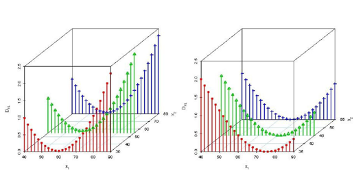
in group A and B separately and the discrepancies are drawn in Figure 1.
- Similar figure can be obtained by deleting
. From this figure the discrepancy is less around the mean of the deleted variable.
Example 2: This is a simulation exercise. Here we have drawn sample of size 159 from bivariate normal distribution and we have used means, variances and correlation coefficient of
and
of the above flu shot data of size 159 for generating the sample. Now using these
and
, we got response that is Y values and thereafter using this whole generated data set we have computed
. Now we have repeated whole process 1000 times and computed means of
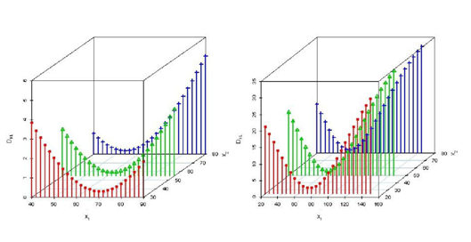
. The mean discrepancies are shown in Figure 2. Here we get the same conclusion as in the data example.
Influence of missing future explanatory variables in log-odds ratio
Here the aim is to detect the predictive influence of a set of missing future explanatory variables in log-odds ratio of logistic model (i). Our interest is to detect the influence of missing future explanatory variables in the six cases pointed out in Section 2. Let in treatment A, r future variables missing from
and s future variables missing from
be denoted by
. Similarly in treatment B, r future missing variables from
and s future variables missing from
be denoted by
. We assume that the errors of models (ii) and (iii) are normally distributed with zero means and variances
and
, respectively. We also assume that the conditional density of
given
is independent of
and
and
given
is independent of
and
, i.e.,
where
denotes the future explanatory variables
without
.
Explanatory variables are continuous
We assume that
s are dependent and the distribution of
is
-dimensional multivariate normal, i.e.
.
The conditional density of
given
is given by
,
Where
and
.
As earlier it is enough to consider Case 5 to see the joint influence of r missing future explanatory variables
of
and s missing future explanatory variables
of
in treatment A. The density of
when
is missing is given by
Where
is the
th component of
and
is the
component of
.
See Bhattacharjee et al11 in this context. Using Taylor's expansion and improper prior density for both
and
, the approximate predictive density of
when
is missing is given by
evaluated at
and
where
is the multiplicative factor for the second order Taylor's approximation. If
’s are independent the corresponding approximate predictive density of
is
evaluated at
and
, where
and
are mean and variance of the ith missing variable and
. Since no future variable is missing in
, the approximate predictive density of
is same as obtained in Section 2. Thus when
’s are dependent the approximate predictive density of log-odds ratio
for
missing is given by
(vi)
Where
and
The Kullback-Leibler9 directed measure of divergence between the predictive densities (iv) when no variable is missing and the predictive density (vi) when
(vii)
If
’s are independent the predictive density of
when
future variables are missing is same as (vi) and the corresponding Kullback-Leibler9 measure
is same as (vii) but replacing
by
in
,
by
in
and
by
in
, where
and
are mean and variance of the ith missing variable.
Explanatory variables are dichotomous
Here we assume that all the explanatory variables are dichotomous and independent. We assume that the errors of models (ii) and (iii) are normally distributed with means zero and variances
and
respectively. To assess the influence of the missing variables in treatment A, we consider that
is distributed as
The density of a future
is
If
future variables are missing in treatment A, then the density of a future
is given by
The predictive density of
when
is missing is given by
(viii)
which is not mathematically tractable. For vague prior densities for
and
and using Taylor's expansion, the approximate predictive density of (viii) is
Since there are no missing variables in
, the density of
is same as that can be obtained in Section 2. Then the predictive density of
is given by
(ix)
Analytical solution of
between the predictive densities (iv) and (ix) is very difficult to obtain but numerical solution can be obtained. In Some situations it is seen that among the explanatory variables, some of the variables are dichotomous and some of the variables are continuous. Among the
-explanatory variables, without loss of generality we assume that the first
are dichotomous and the remaining last
are continuous variables. We also assume that out of l dichotomous future variables last d variables are missing and out of
continuous future variables last g variables are missing. Then the predictive density of future log-odds ratio
when d dichotomous and g continuous variables are missing is given by
(x)
Again, analytical solution of
between the predictive densities (iv) and (x) is very difficult but we can obtain its numerical solution. In similar way we can derive the predictive density of future log-odds ratio when some future variables are missing in treatment B.
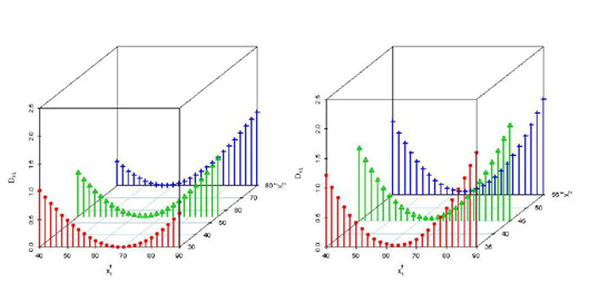
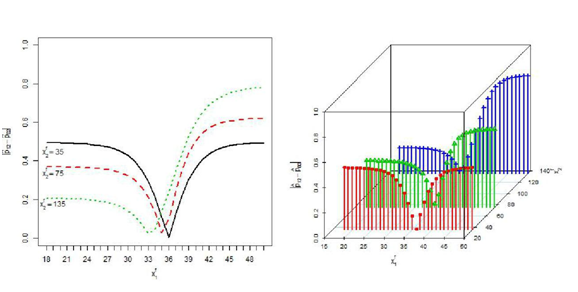
Example 1 revisited: This example is based on the flu shot data of Example 1. From Figure 3 we have observed same as Examples 1 and 2 that the discrepancies are less around the mean of the missing variables. Moreover we have observed from Figures 1 and 3 that the discrepancies of the missing variables are less as compared to the discrepancies of the deleted variables.
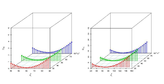
Example 2 revisited: This example is based on the simulation data of Example 2 and here we have also got same conclusion as Example 1 revisited (Figures 2 & 4).

Group A Group B
Figure 1 Three dimensional scatter plots based on real data for DKL
when x1 is deleted.

Group A Group B
Figure 2 Three dimensional scatter plots based on simulated data for DKL
when x1 is deleted.

Group A Group B
Figure 3 Three dimensional scatter plots based on real data for DKL
when x
f1 is missing.

Group A Group B
Figure 4 Three dimensional scatter plots based on simulated data for DKL
when x
f1 is missing.
Examples 1 and 2 revisited: In this example, we have used
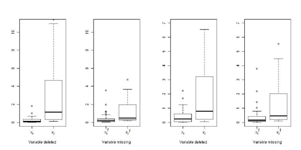
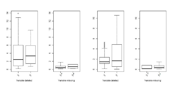
values for real data for drawing box plots for each cases (deleted and missing). From Figure 5, we have observed that x2 is more in uential than x1. Moreover the discrepancies are much less in missing case than deleted case. We have got same result in simulation study and are illustrated in Figure 6.
Treatment A Treatment B
Figure 5 Box plot for DKL based on real data.
Treatment A Treatment B
Figure 6 Box plot for DKL based on simulated data.
Evaluation of predictive probability of a logistic model
We consider the logistic model as
The probability that a future response yf will be a success is given by
We assume that the conditional density of xf(r) given xf is independent of,
where xf denotes the future explanatory variables without variables xf(r). Then predictive probabilities of yf will be a success for models are given by
and
respectively. Simple analytically tractable priors are not available here. Numerical integration techniques might be used for some specified priors to approximate
and
, respectively.
Normal approximation for the posterior density
Let us suppose that the sample size is large. Lindley12 stated that the posterior density
may then be well approximated by its asymptotic normal form as
where
is the maximum likelihood estimate of β, ∑ = (-H)-1 and H is the Hessian of log L(β) evaluated at .
For the logistic model (xi), the Hessian H=(hji(
)) evaluated at is given by
Where xij is the jth component of
with
= 1. For given
will have approximately a posteriori a normal distribution with mean
=
and variance
, and with probability density function
. Using the transformation we can approximate
by
Analytical evaluation of (4.1) is very di cult. We can however evaluate then by numerical integration techniques viz Gauss-Hermite Quadrature Abramowitz and Stegun,13 Normal approximation Cox,14 Laplace's approximation de Bruijn.15
If the sample size is small, the posterior normality assumption may not be accurate. Therefore, we consider Flat prior approximation Tierney and Kadane16 as an alternative approach using the Laplace's method for integrals.
Effect of the variables
Here we assume that the future variables
are dependent and the density of
is p-dimensional multivariate normal i.e.
The conditional density of
for given
is
The probability of
as a success when
is missing given by
(Say)
Then the predictive probability of
as a success when
is missing given by
(xii)
The integral in (Xii) can be evaluated as the integral in (Xi) using Taylor's and Laplace's approximations.
If, instead, the future variables
,…,
are independently and normally distributed with mean
and variance (i = 1, 2, … , k), then the conditional density of
is
.
Consequently, we get
(Say)
See Aitchison and Begg17 in this context. Again,
Variables
are dichotomous
Here we assume that the variables
are independent and they can take only two values 0 or 1. We also assume that
is distributed as
If
is missing the probability of
as a success is given by
(Say).
The predictive probability of
as a success when
is missing is given by
(xiii)
If the sample size is large, assuming the normality assumption for the posterior density we can approximate (xiii) using Taylor's theorem, Laplace's method and normal approximation.
Example: one variable case
Here we consider two different logistic models based on any single variable either
or
. We want to measure the discrepancies between the predictive probability
, based on a single variable
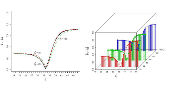
when
is known, and the predictive probability
, based on xi alone when
is missing, to assess the influence of the missing variable
, i = 1, 2. The predictive probability
is determined using quadrature approximation and the predictive probability
is determined using second order Taylor's approximation.
We assume that the marginal densities of the future variables
and
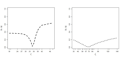
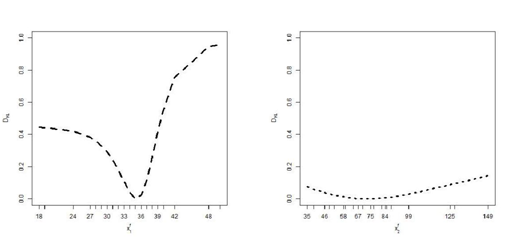
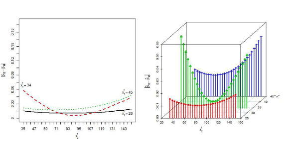
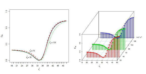
are normal with means 33.35, 78.24 and variances 65.39, 1827.0 respectively, where means and variances are the estimated sample means and sample variances from the observed data. We employ the absolute difference of probabilities and Kullback-Leibler divergence measure to assess the influence of the missing variable. The discrepancies are drawn in Figure 7. Here we see that the discrepancies due to missing
in the predictive probability based on
are very large compared to the discrepancies due to missing
in the predictive probability based on
. The discrepancies are less around the mean of the missing variable.

x1 fis missing x2f is missing
Kullback-Leibler directed divergence D_{KL}

x1 fis missing x2f is missing
Figure 7 Absolute difference
Example: two-variable case
Now we consider that the predictive probability based on two variables
and
when both
and
are known is denoted by
and the predictive probability
,
,
and
based on
and
when any future variable is missing. "0" indicates missing variable. Here also the predictive probability
is determined using quadrature approximation and predictive probabilities
,
and
are determined using second order Taylor's approximation. Here we assume that the joint density of
and
is bivariate normal with correlation coefficient 0.33 which is the estimated sample correlation coefficient from the observed data. The absolute differences of the two predictive probabilities
and
when
is missing and the absolute differences of the two predictive probabilities
and
when
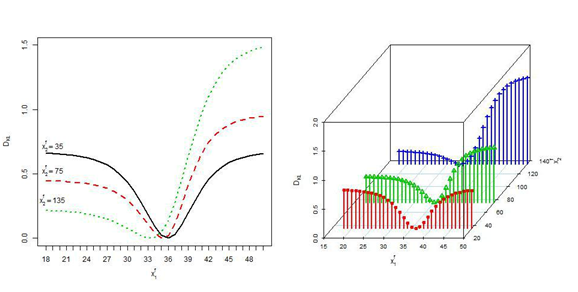
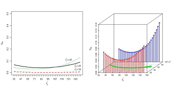
is missing are drawn in Figure 8. Kullback-Leibler directed divergence DKL are drawn in Figure 9. The discrepancies when
is missing and for different given values of the other variable for both the cases are close together since the correlation between
and
are very small. The discrepancies due to missing
are very large compared to missing
except near the mean of the missing variable. If both
and
are missing the discrepancies are drawn in Figure 10. These discrepancies are very similar to the discrepancies due to missing
alone in the predictive probability based on
and
since the contribution of
is negligible.
x1f is missing
xf2 is missing
Figure 8 Absolute difference
xf1 is missing
Kullback-Leibler directed divergence DKL
xf2 is missing
Figure 9 Kullback-Leibler directed divergence DKL
Absolute difference
.
Kullback-Leibler directed divergence DKL
Figure 10 X1f and X2ffare both missing.
Concluding remarks
In our present study we have observed that the discrepancies are minimum around the mean of the deleted variables as well as the mean of the missing future variables in both the logistic model and the log-odds ratio; the discrepancies are larger if the deleted or missing variables are more influential; the discrepancies in the deleted case are higher than the missing case.
In this present paper we studied the important problem of predictive influence of variables on the log odds ratio under a Bayesian set up. The treatment difference
Or the risk of ratio
can also be studied along the same lines.
We have also considered the influence of missing future explanatory variables in a logistic model. Influence of missing future explanatory variables in a Probit and complementary log-log models can also be studied in similar fashion.
Acknowledgments
Conflicts of interest
References
- Breslow N. Odds ratio estimators when the data are sparse. Biometrika. 1981;68:73–84.
- Bohning D, Kuhnert, Rattanasiri S, et al. Meta–analysis of binary data using pro le likelihood. 1st ed. A Chapman and Hall CRC Interdisciplinary Statistic. 2008.
- Pregibon D. Logistic regression diagnostics. Annals of Statistics. 1981;9:705–724.
- Cook, R Dennis, Weisberg, et al. Residuals and Influence in Regression. USA: New York: Chapman and Hall. 1982.
- Johnson W. Influence measures for logistic regression: Another point of view. Biometrika. 1985;72(1):59–65.
- Bhattacharjee SK, Dunsmore IR. The influence of variables in a logistic model. Biometrika. 1991;78(4):851–856.
- Mercier C, Shelley MC, Rimkus J, et al. Age and Gender as Predictors of Injury Severity in Head–on Highway Vehicular Collisions. The 76th Annual Meeting , Transportation Research Board, Washington, USA. 1997.
- Zellner D, Keller F, Zellner GE. Variable selection in logistic regression models. Communications in Statistics. 2004;33(3):787–805.
- Kullback S, Leibler R A. On information and sufficiency. Ann Math Statist. 1951;22:79–86.
- S Rao Jammalamadaka, Tiwari RC, Chib Siddhartha. Bayes prediction in the linear model with spherically symmetric errors. Economics Letters. 1987;24:39–44.
- Bhattacharjee SK, Shamiri A, Sabiruzzaman Md, et al. Predictive Influence of Unavailable Values of Future Explanatory Variables in a Linear Model. Communications in Statistics – Theory and Methods. 2011;40:4458–4466.
- Lindley D V. The use of prior probability distributions in statistical inference and decisions. Proc. 4th Berkeley Symp. 1961;1:453–468.
- Abramowitz M, Stegun I A . Handbook of Mathematical Functions. USA: National Bureau of Standards. 1966.
- Cox DR. Binary regression. UK: London: Chapman and Hall. 1970.
- De Bruijn N C. Asymptotic Methods in Analysis. Amsterdam, North–Holland. 1961.
- Tierney L, Kadane, Joseph B, et al. Accurate approximations for posterior moments and marginal densities. Journal of the American Statistical Association. 1986;81(393):82–86.
- Aitchison J, Bagg CB (1976) Statistical diagnosis when basic cases are not classified with certainty. Biometrika 63: 1-12.
- Logistic Regression Example with Grouped Data. Regression FluShots, University of North Florida.
- Bhattacharjee SK, Dunsmore IR. The predictive influence of variables in a normal regression model. J Inform Optimiz Sci. 1995;16(2):327–334.

©2017 Bhattacharjee, et al. This is an open access article distributed under the terms of the,
which
permits unrestricted use, distribution, and build upon your work non-commercially.


