
Research Article Volume 3 Issue 1
On two - parameter lindley distribution and its applications to model lifetime data
Rama Shanker,1  Hagos Fesshaye,2 Shambhu Sharma3
1Department of Statistics, Eritrea Institute of Technology, Eritrea
2Department of Economics, College of Business and Economics, Eritrea
3Department of Mathematics, Dayalbagh Educational Institute, India
Correspondence: Rama Shanker, Eritrea Institute of Technology, Asmara, Eritrea
Received: October 28, 2015 | Published: January 2, 2016
Citation: Shanker R, Fesshaye H, Sharma S. On two - parameter lindley distribution and its applications to model lifetime data. Biom Biostat Int J. 2016;3(1):9-15. DOI: 10.15406/bbij.2016.03.00056
Download PDF
Abstract
In this paper some of the important mathematical properties including moment generating function, mean deviations, order statistics, Bonferroni and Lorenz curves, Renyi entropy and stress strength reliability of two-parameter Lindley distribution (TPLD) of Shanker & Mishra1 have been discussed. Its goodness of fit over exponential and Lindley distributions have been illustrated with some real lifetime data-sets and found that TPLD is preferable over exponential and Lindley distributions for modeling lifetime data-sets.
Keywords: mean deviations; order statistics, bonferroni and lorenz curves, entropy, stress-strength reliability, goodness of fit
Introduction
The probability density function (p.d.f.) and the cumulative distribution function (c.d.f.) of distribution, introduced in the context of Bayesian analysis as a counter example of fiducial statistics, are given by
(1.1)
(1.2)
The detailed study about its mathematical properties, estimation of parameter and application showing the superiority of Lindley distribution over exponential distribution for the waiting times before service of the bank customers has been done by Ghitany et al.2 The Lindley distribution has been generalized extended and modified by different researchers including1,3-19 are some among others.
The probability density function (p.d.f.) and cumulative distribution function (c.d.f) of two-parameter Lindley distribution (TPLD) of Shanker & Mishra1 are given by
(1.3)
(1.4)
At
, both (1.3) and (1.4) reduce to the corresponding expressions (1.1) and (1.2) of Lindley distribution. The first two moments about origin and the variance of TPLD of Shanker & Mishra1 are given by
(1.5)
(1.6)
(1.7)
At
, these moments reduce to the corresponding moments of Lindley distribution. Shanker & Mishra1 have derived and discussed some of its mathematical properties such as shape, moments, coefficient of variation, coefficient of skewness and kurtosis, hazard rate function, mean residual life function and stochastic orderings. They have also discussed the estimation of its parameters using maximum likelihood estimation and method of moments and its goodness of fit over Lindley distribution. It has been observed that many important mathematical properties of this distribution have not been studied.
In the present paper some of the important mathematical properties including moment generating function, mean deviations, order statistics, Bonferroni and Lorenz curves, Renyi entropy and stress strength reliability of TPLD of Shanker & Mishra1 have been derived and discussed. Its goodness of fit over exponential and Lindley distributions have been illustrated with some real lifetime data-sets and found that TPLD gives better fit than exponential and Lindley distributions.
Moment generating function
The moment generating function,
of TPLD (1.3) can be obtained as
It can be easily seen that the expression for
obtained as the coefficient of
is given as
For
,
reduces to the corresponding
of Lindley distribution.
Mean deviations
The amount of scatter in a population is measured to some extent by the totality of deviations usually from mean and median. These are known as the mean deviation about the mean and the mean deviation about the median defined by
and
, respectively, where
and
. The measures
and
can be calculated using the relationships
(3.1)
and
(3.2)
Using p.d.f. (1.3), and expression for mean of two-parameter Lindley distribution, we have
(3.3)
Using expressions from (3.1), (3.2) and (3.3), and little algebraic simplification, the mean deviation about mean,
and the mean deviation about median,
of TPLD (1.3) are obtained as
(3.4)
and
(3.5)
It can be easily seen that expressions (3.4) and (3.5) of TPLD (1.3) reduce to the corresponding expressions of Lindley distribution at
.
Order statistics
Let
be a random sample of size from two-parameter Lindley distribution (1.3). Let
denote the corresponding order statistics. The p.d.f. and the c.d.f. of the
th order statistic, say
are given by
and
respectively, for
Thus, the p.d.f. and the c.d.f of the th order statistics of TPLD (1.3) are obtained as
and
It can be easily verified that the expressions for the p.d.f. and c.d.f. of the th order statistics of TPLD (1.3) reduce to the expressions for the p.d.f. and c.d.f. of the th order statistics of Lindley distribution at
Bonferroni and lorenz curves
The Bonferroni and Lorenz curves20 and Bonferroni and Gini indices have applications not only in economics to study income and poverty, but also in other fields like reliability, demography, insurance and medicine. The Bonferroni and Lorenz curves are defined as
(5.1)
(5.2)
respectively or equivalently
(5.3)
and
(5.4)
respectively, where
and
.
The Bonferroni and Gini indices are thus defined as
(5.5)
and
(5.6)
respectively.
Using p.d.f. (1.3), we get
(5.7)
Now using equation (5.7) in (5.1) and (5.2), we get
(5.8)
and
(5.9)
Now using equations (5.8) and (5.9) in (5.5) and (5.6), the Bonferroni and Gini indices of TPLD (1.3) are obtained as
(5.10)
(5.11)
The Bonferroni and Gini indices of Lindley distribution are particular cases of the Bonferroni and Gini indices (5.10) and (5.11) of TPLD (1.3) for
.
Renyi entropy
An entropy of a random variable is a measure of variation of uncertainty. A popular entropy measure is Renyi entropy.21 If is a continuous random variable having probability density function
, then Renyi entropy is defined as
where
.
Thus, the Renyi entropy for TPLD (1.3) can be obtained as
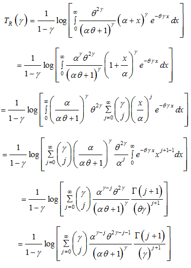
The Renyi entropy of Lindley distribution is a particular case of the Renyi entropy TPLD at
.
Stress-strength reliability
The stress- strength reliability describes the life of a component which has random strength that is subjected to a random stress . When the stress applied to it exceeds the strength, the component fails instantly and the component will function satisfactorily till
. Therefore,
is a measure of component reliability and in statistical literature it is known as stress-strength parameter. It has wide applications in almost all areas of knowledge especially in engineering such as structures, deterioration of rocket motors, static fatigue of ceramic components, aging of concrete pressure vessels etc.
Let
and
be independent strength and stress random variables having TPLD (1.3) with parameter
and
respectively. Then the stress-strength reliability
is obtained as
The expression of stress-strength reliability of Lindley distribution is a particular case of the expression of stress-strength reliability of TPLD (1.3) at
.
Estimation of parameters
- Method of moment estimate of parameters
The TPLD (1.3) has two parameters to be estimated and so the first two moments about origin are required to estimate parameters. Using the first two moments about origin, we have
(8.1.1)
Taking
, we get
This gives a quadratic equation in
as
(8.1.2)
Replacing the first and second moments about origin
and
by their respective sample moments, an estimate of
can be obtained and substituting the value of
in equation (8.1.2), an estimate of can be obtained. Substituting this estimate of in the expression for the mean of TPLD (1.3), moment estimate
of
can be obtained as
(8.1.3)
Finally, moment estimate
of
can be obtained as
(8.1.3)
Finally, moment estimate
of
can be obtained as
b. Maximum likelihood estimate of parameters
Let
be a random sample from TPLD (1.3). Let
be the observed frequency in the sample corresponding to
such that
, where
is the largest observed value having non-zero frequency. The likelihood function,
of TPLD (1.3) is given by
(8.2.1)
The log likelihood function is thus obtained as
(8.2.2)
where
is the sample mean.
The two log likelihood equations are obtained as
It can be easily seen that equation (8.2.3) gives
, mean of TPLD. The equations (8.2.3) and (8.2.4) do not seem to be solved directly. However, Fisher’s scoring method can be applied to solve these equations iteratively. We have
(8.2.6)
(8.2.7)
The maximum likelihood estimates of parameters are the solution of the following equations
where
are initial values of
as given by the method of moments. These equations are solved iteratively till sufficiently close estimates of
are obtained.
Applications of two-parameter Lindley distribution
The two-parameter Lindley distribution (TPLD) has been fitted to a number of lifetime data- sets. In this section, we present the fitting of two-parameter Lindley distribution to five real lifetime data-sets and compare its goodness of fit with the one parameter exponential and Lindley distributions data sets (1-5).
1.1 |
1.4 |
1.3 |
1.7 |
1.9 |
1.8 |
1.6 |
2.2 |
1.7 |
2.7 |
4.1 |
1.8 |
1.5 |
1.2 |
1.4 |
3 |
1.7 |
2.3 |
1.6 |
2 |
|
|
|
|
Data set 1: This data set represents the lifetime’s data relating to relief times (in minutes) of 20 patients receiving an analgesic and reported by Gross et al.22
18.83 |
20.8 |
21.657 |
23.03 |
23.23 |
24.05 |
24.321 |
25.5 |
25.52 |
25.8 |
26.69 |
26.77 |
26.78 |
27.05 |
27.67 |
29.9 |
31.11 |
33.2 |
33.73 |
33.76 |
33.89 |
34.76 |
35.75 |
35.91 |
36.98 |
37.08 |
37.09 |
39.58 |
44.045 |
45.29 |
45.381 |
|
|
|
|
|
Data set 2: This data set is the strength data of glass of the aircraft window reported by Fuller et al.23
0.8 |
0.8 |
1.3 |
1.5 |
1.8 |
1.9 |
1.9 |
2.1 |
2.6 |
2.7 |
2.9 |
3.1 |
3.2 |
3.3 |
3.5 |
3.6 |
4 |
4.1 |
4.2 |
4.2 |
4.3 |
4.3 |
4.4 |
4.4 |
4.6 |
4.7 |
4.7 |
4.8 |
4.9 |
4.9 |
5 |
5.3 |
5.5 |
5.7 |
5.7 |
6.1 |
6.2 |
6.2 |
6.2 |
6.3 |
6.7 |
6.9 |
7.1 |
7.1 |
7.1 |
7.1 |
7.4 |
7.6 |
7.7 |
8 |
8.2 |
8.6 |
8.6 |
8.6 |
8.8 |
8.8 |
8.9 |
8.9 |
9.5 |
9.6 |
9.7 |
9.8 |
10.7 |
10.9 |
11 |
11 |
11.1 |
11.2 |
11.2 |
11.5 |
11.9 |
12.4 |
12.5 |
12.9 |
13 |
13.1 |
13.3 |
13.6 |
13.7 |
13.9 |
14.1 |
15.4 |
15.4 |
17.3 |
17.3 |
18.1 |
18.2 |
18.4 |
18.9 |
19 |
19.9 |
20.6 |
21.3 |
21.4 |
21.9 |
23 |
27 |
31.6 |
33.1 |
38.5 |
|
|
|
|
|
|
|
|
Data set 3: This data set represents the waiting times (in minutes) before service of 100 Bank customers and examined and analyzed by Ghitany et al.2 for fitting the Lindley24 distribution.
0.55 |
0.93 |
1.25 |
1.36 |
1.49 |
1.52 |
1.58 |
1.61 |
1.64 |
1.68 |
1.73 |
1.81 |
2 |
0.74 |
1.04 |
1.27 |
1.39 |
1.49 |
1.53 |
1.59 |
1.61 |
1.66 |
1.68 |
1.76 |
1.82 |
2.01 |
0.77 |
1.11 |
1.28 |
1.42 |
1.5 |
1.54 |
1.6 |
1.62 |
1.66 |
1.69 |
1.76 |
1.84 |
2.24 |
0.81 |
1.13 |
1.29 |
1.48 |
1.5 |
1.55 |
1.61 |
1.62 |
1.66 |
1.7 |
1.77 |
1.84 |
0.84 |
1.24 |
1.3 |
1.48 |
1.51 |
1.55 |
1.61 |
1.63 |
1.67 |
1.7 |
1.78 |
1.89 |
|
|
|
|
|
|
|
|
|
Data set 4: The data set represents the strength of 1.5cm glass fibers measured at the National Physical Laboratory, England. Unfortunately, the units of measurements are not given in the paper, and they are taken from Smith & Naylor25
17.88 |
28.92 |
33 |
41.52 |
42.12 |
45.6 |
48.8 |
51.84 |
51.96 |
54.12 |
55.56 |
67.8 |
68.44 |
68.64 |
68.88 |
84.12 |
93.12 |
98.64 |
105.12 |
105.84 |
127.92 |
128.04 |
173.4 |
|
Data set 5: The data set is from Lawless.26 The data given arose in tests on endurance of deep groove ball bearings. The data are the number of million revolutions before failure for each of the 23 ball bearings in the life tests and they are:
In order to compare distributions,
, AIC (Akaike Information Criterion), AICC (Akaike Information Criterion Corrected), BIC (Bayesian Information Criterion), K-S Statistics (Kolmogorov-Smirnov Statistics) for five real data - sets have been computed (Table 1). The formulae for computing AIC, AICC, BIC, and K-S Statistics are as follows:
|
Model |
Estimate of Parameters |
— 2ln L |
AIC |
AICC |
BIC |
K-S
Statistics |
|
|
Data 1 |
Lindley |
0.816118 |
|
60.50 |
62.50 |
62.72 |
63.49 |
0.341 |
|
Exponential
TPLD |
0.526316
1.545110 |
— 0.31285 |
65.67
40.71 |
67.67
44.71 |
67.90
45.41 |
68.67
46.70 |
0.389
0.204 |
Data 2 |
Lindley |
0.062988 |
|
253.99 |
255.99 |
256.13 |
257.42 |
0.333 |
|
Exponential
TPLD |
0.032455
0.103985 |
— 5.25330 |
274.53
231.82 |
276.53
235.82 |
276.67
236.25 |
277.96
238.69 |
0.426
0.298 |
Data 3 |
Lindley |
0.186571 |
|
638.07 |
640.07 |
640.12 |
642.68 |
0.058 |
|
Exponential
TPLD |
0.101245
0.196210 |
0.337078 |
658.04
635.75 |
660.04
639.75 |
660.08
639.87 |
662.65
639.75 |
0.163
0.040 |
Data 4 |
Lindley |
0.996116 |
|
162.56 |
164.56 |
164.62 |
166.70 |
0.371 |
|
Exponential
TPLD |
0.663647
2.146474 |
0.257373 |
177.66
91.56 |
179.66
95.56 |
179.73
95.63 |
181.80
97.36 |
0.402
0.361 |
Data 5 |
Lindley |
0.027321 |
|
231.47 |
233.47 |
233.66 |
234.61 |
0.149 |
|
Exponential
TPLD |
0.013845
0.035434 |
10.12355 |
242.87
223.52 |
244.87
227.52 |
245.06
228.12 |
246.01
229.79 |
0.263
0.098 |
Table 1 MLE’s, — 2ln L, AIC, AICC, BIC, K-S Statistics of the fitted distributions of data sets 1-5
,
,
and
, where
= the number of parameters,
= the sample size and
is the empirical distribution function.
The best distribution corresponds to lower
, AIC, AICC, BIC, and K-S statistics.
Conclusion
In the present paper some of the important mathematical properties including moment generating function, mean deviations, order statistics, Bonferroni and Lorenz curves, entropy and stress strength reliability of two-parameter Lindley distribution (TPLD) of Shanker & Mishra
1 have been derived and discussed. The distribution has been fitted to some real lifetime data-sets to test its goodness of fit over exponential and Lindley distributions. It is obvious from the fitting of TPLD that it gives better fitting than exponential and Lindley distributions and hence TPLD is preferable over exponential and Lindley distributions for modeling lifetime data-sets from different fields of knowledge.
Acknowledgments
Conflicts of interest
References
- Shanker R, Mishra A. A two-parameter Lindley distribution. Statistics in Transition-new series. 2013A;14(1): 45–56.
- Ghitany ME, Atieh B, Nadarajah S. Lidley distribution and its Application. Mathematics Computing and Simulation. 2008;78(4):493–506.
- Zakerzadeh H, Dolati A. Generalized Lindley distribution. Journal of Mathematical extension. 2009;3(2):13–25.
- Nadarajah S, Bakouch HS, Tahmasbi R. A generalized Lindley distribution. Sankhya Series. 2011;73(2):331–359.
- Deniz E, Ojeda E. The discrete Lindley distribution-Properties and Applications. Journal of Statistical Computation and Simulation. 2011;81(11):1405–1416.
- Bakouch HS, Al Zaharani B, Al Shomrani A, et al. An extended Lindley distribution. Journal of the Korean Statistical Society. 2012;41(1):75–85.
- Shanker R, Mishra A. A quasi Lindley distribution. African Journal of Mathematics and Computer Science Research. 2013B;6(4):64–71.
- Shanker R, Sharma S, Shanker R. A two-parameter Lindley distribution for modelling waiting and survival times data. Applied Mathematics. 2013;4(2):363–368.
- Elbatal I, Merovi F, Elgarhy M. A new generalized Lindley distribution. Mathematical theory and Modelling. 2013;3(13):30–47.
- Ghitany M, Al Mutairi D, Balakrishnan N, et al. Power Lindley distribution and associated inference. Computational Statistics and Data Analysis. 2013;64:20–33.
- Merovci F. Transmuted Lindley distribution. International Journal of Open Problems in Computer Science and Mathematics. 2013;6(2):63–72.
- Liyanage GW, Pararai M. A generalized Power Lindley distribution with applications. Asian journal of Mathematics and Applications. 2014;1–23.
- Ashour S, Eltehiwy M. Exponentiated Power Lindley distribution. Journal of Advanced Research. 2014;6(6):895–905.
- Oluyede BO, Yang T. A new class of generalized Lindley distribution with applications. Journal of Statistical Computation and Simulation. 2014;85(10):2072–2100.
- Singh SK, Singh U, Sharma VK. The Truncated Lindley distribution-inference and Application. Journal of Statistics Applications & Probability. 2014;3(2):219–228.
- Sharma V, Singh S, Singh U. The inverse Lindley distribution-A stress-strength reliability model with applications to head and neck cancer data. Journal of Industrial &Production Engineering. 2015;32(3):162–173.
- Shanker R, Hagos F, Sujatha S. On modeling of Lifetimes data using exponential and Lindley distributions. Biometrics & Biostatistics International Journal. 2015;2(5):1–9.
- Alkarni S.Extended Power Lindley distribution-A new Statistical model for non-monotone survival data. European journal of statistics and probability. 2015;3(3):19–34.
- Pararai M, Liyanage GW, Oluyede BO. A new class of generalized Power Lindley distribution with applications to lifetime data. Theoretical Mathematics &Applications. 2015;5(1):53–96.
- Bonferroni CE. Elementi di Statistca generale. Seeber, Firenze, Itlay. 1930.
- Renyi A. On measures of entropy and information in proceedings of the 4th Berkeley symposium on Mathematical Statistics and Probability. University of California press, Berkeley, USA, 1961;1:547–561.
- Gross AJ, Clark VA. Survival Distributions Reliability Applications in the Biometrical Sciences. New York, USA. John Wiley. 1975.
- Fuller EJ, Frieman S, Quinn J, et al. Fracture mechanics approach to the design of glass aircraft windows: A case study. SPIE Proc. 1994; 2286:419–430.
- Lindley DV. Fiducial distributions and Bayes’ theorem. Journal of the Royal Statistical Society. Series B. 1958;20(1):102–107.
- Smith RL, Naylor JC. A comparison of Maximum likelihood and Bayesian estimators for the three parameter Weibull distribution. Applied Statistics. 1987;36(3):358–369.
- Lawless JF. Statistical models and methods for lifetime data. New York, USA; John Wiley and Sons. 1982.

©2016 Shanker, et al. This is an open access article distributed under the terms of the,
which
permits unrestricted use, distribution, and build upon your work non-commercially.
