
Research Article Volume 4 Issue 2
On discrete three parameter burr type XII and discrete lomax distributions and their applications to model count data from medical science
Para BA,
Regret for the inconvenience: we are taking measures to prevent fraudulent form submissions by extractors and page crawlers. Please type the correct Captcha word to see email ID.

Jan TR
Department of statistics, University of Kashmir, India
Correspondence: Bilal Ahmad Para, Department of statistics, University of Kashmir, Srinagar, J&K(India)-192301, Srinagar, Jammu and Kashmir, India
Received: May 19, 2016 | Published: July 23, 2016
Citation: Para BA, Jan TR. On discrete three parameter burr type xii and discrete lomax distributions and their applications to model count data from medical science. Biom Biostat Int J. 2016;4(2):70-82. DOI: 10.15406/bbij.2016.04.00092
Download PDF
Abstract
In this paper we propose a discrete analogue of three parameter Burr type XII distribution and discrete Lomax distribution as new discrete models using the general approach of discretization of continuous distribution. The models are plausible in modeling discrete data and exhibit both increasing and decreasing hazard rates. We shall first study some basic distributional and moment properties of these new distributions. Then, certain structural properties of the distributions such as their unimodality, hazard rate behaviors and the second rate of failure functions are discussed. Developing a discrete versions of three parameter Burr type XII and Lomax distributions would be helpful in modeling a discrete data which exhibits heavy tails and can be useful in medical science and other fields. The equivalence of discrete three parameter Burr type XII (DBD-XII) and continuous Burr type XII (BD-XII) distributions has been established and similarly characterization results have also been made to establish a direct link between the discrete Lomax distribution and its continuous counterpart. Various theorems relating a three parameter discrete Burr type XII distribution and discrete Lomax distribution with other statistical distributions have also been proved. Finally, the models are examined with an example data set originated from a study,1,2 data set of counts of cysts of kidneys using steroids and compared with the classical models.
Keywords: discrete lomax distribution, AIC, ML estimate, failure rate, medical sciences, index of dispersion
Introduction
Statistical models describe a phenomenon in the form of mathematical equations. Plethora of continuous lifetime models in reliability theory is now available in the subject to portray the survival behavior of a component or a system. Most of the lifetimes are continuous in nature and hence many continuous life distributions have been studied in literature Kapur & Lamberson,3 Lawless4 and Sinha.5 However, it is sometimes impossible or inconvenient in life testing experiments to measure the life length of a device on a continuous scale. Equipment or a piece of equipment operates in cycles and experimenter observes the number of cycles successfully completed prior to failure. A frequently referred example is copier whose life length would be the total number of copies it produces. Another example is the lifetime of an on/off switching device is a discrete random variable, or life length of a device receiving a number of shocks it sustain before it fails. Or in case of survival analysis, we may record the number of days of survival for lung cancer patients since therapy, or the times from remission to relapse are also usually recorded in number of days. In the recent past special roles of discrete distribution is getting recognition from the analysts in the field of reliability theory. In this context, the well known distributions namely geometric and negative binomial are known discrete alternatives for the exponential and gamma distributions, respectively. It is also well known that these discrete distributions have monotonic hazard rate functions and thus they are unsuitable for some situations. Fortunately, many continuous distributions can be discretized. As mentioned earlier, the discrete versions of exponential and gamma are geometric and negative binomial. There are three discrete versions of the continuous Weibull distribution.14 The discrete versions of the normal and rayleigh distributions were also proposed by Roy.6,7 Discrete analogues of two parameter Burr XII and Pareto distributions were also proposed by Krishna & Punder.8 Recently discrete inverse Weibull distribution was studied,9 which is a discrete version of the continuous inverse Weibull variable, defined as
where
denotes the continuous Weibull random variable. Para & Jan10 proposed a discrete version of two parameter Burr type III distribution as a reliability model to fit a range of discrete life time data. Deniz & Ojeda11 introduced a discrete version of Lindley distribution by discretizing the continuous failure model of the Lindley distribution. Also, a compound discrete Lindley distribution in closed form is obtained after revising some of its properties. Nekoukhou et al.12 presented a discrete analog of the generalized exponential distribution, which can be viewed as another generalization of the geometric distribution, and some of its distributional and moment properties were discussed.
In the present paper we propose a three parameter discrete Burr type XII (DBD-XII) model and a two parameter discrete Lomax model as there is a need to find more plausible discrete life time distributions or survival models in medical science and other fields, to fit to various life time data. The model has a flexible index of dispersion which broaden its range to fit a data sets arising in medical science/biological science, engineering, finance etc.
Burr13 introduced a family of distributions includes twelve types of cumulative distribution functions, which yield a variety of density shapes. The two important members of the family are Burr type III and Burr type XII distributions. Types III and XII are the simplest functionally and therefore, the two distributions are the most desirable for statistical modeling.
A continuous random variable X is said to follow a three parameter Burr type XII distribution if its pdf is given by
and its cumulative distribution function is given by
When c=1, the three parameter Burr type XII distribution becomes Lomax distribution with pdf given
and its cumulative distribution function is given by
Figures 1-4 gives the pdf plot for three parameter Burr type XII distribution and Lomax distribution for different values of parameters. Figure 3 & Figure 4 are especially for Lomax distribution. It is evident that the distribution of the rv X exhibit a right skewed nature.
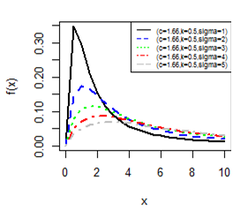
Figure 1 pdf plot for BD-XII (c,k,γ)
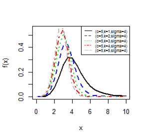
Figure 2 pdf plot for BD-XII (c,k,γ)
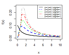
Figure 3 pdf plot for BD-XII (c,k, γ).
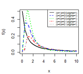
Figure 4 PDF plot for BD-XII (c, k, γ).
The various reliability measures of three parameter Burr type XII random variable X are given by
- Survival function
- The failure rate is given by
- The second rate of failure is given by
- The rth moment is
Where
,
The convergence of the rth moment is only possible if ck>r
Three parameter discrete Burr type XII and discrete lomax model
Roy14 pointed out that the univariate geometric distribution can be viewed as a discrete concentration of a corresponding exponential distribution in the following manner:
When x = 0, 1, 2,…..
Where X is discrete random variable following geometric distribution with probability mass functions as
x = 0,1,2,…….
Where s(x) represents the survival function of an exponential distribution of the form
clearly
.
Thus, one to one correspondence between the geometric distribution and the exponential distribution can be established, the survival functions being of the same form.
The general approach of dicretising a continuous variable is to introduce a greatest integer function of X i.e., [X] (the greatest integer less than or equal to X till it reaches the integer), in order to introduce grouping on a time axis.
A discrete Burr type XII variable, dX can be viewed as the discrete concentration of the continuous Burr type XII variable X, where the corresponding probability mass function of dX can be written as:
The probability mass function takes the form
(3.1)
Where
And the cumulative distribution function is given by
Where
(3.2)
When c=1, the three parameter discrete Burr type XII distribution becomes discrete Lomax distribution with pdf and cdf given by
(3.3)
Where
Where
(3.4)
The quantile functions for three parameter discrete Burr type XII and discrete Lomax distributions can be obtained by inverting (3.2) and (3.4) respectively.
for DBD-XII and
for DLomax distribution.
Where
Where [ ] denotes the greatest integer function (the largest integer less than or equal). In particular, the median can be written as
for three parameter discrete Burr type XII distribution and for discrete Lomax distribution the median is
Where
The parameter
completely determines the pmf (3.1) at x = 0 and = 1. It should be also noted that in this case the p(x) is always monotonic decreasing for x = 1,2,3,4,….
When
Where
Where
otherwise it is no longer monotonic decreasing but is unimodal, having a mode at
i.e., it takes a jump at x=1 and then decreases for all
. Figures 5-10 exhibit a graphical overview of the pmf plot for both three parameter discrete Burr type XII and discrete Lomax models for different values of parameters.
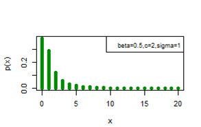
Figure 5 pmf plot for DBD-XII (β, c, γ).
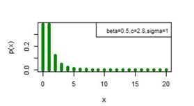
Figure 6 pmf plot for DBD-XII (β, c, γ).
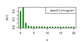
Figure 7 pmf plot for DBD-XII (β, c, γ).
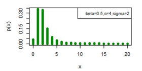
Figure 8 pmf plot for DBD-XII (β, c, γ).
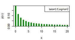
Figure 9 pmf plot for DLomax (β, γ).
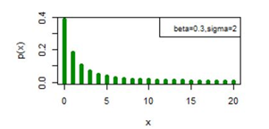
Figure 10 pmf plot for DLomax (β, γ).
In addition, the modal value of three parameter discrete Burr type XII distribution,
is given by
, in case when c>1 [if
, then the distribution is monotonic decreasing for all x=0,1,2,…..] , the value of c plays a very important role in determining the shape of the cdf curve , the lower the value of c , the sharper the fall of cdf curve, while lower the value of k parameter, the sharper the initial rise of the cdf curve.
When
, the distribution of three parameter discrete Burr type XII model can attain model value other than at x=1 and x=0 also. Figures 11-13 provides display of pmf plot when the model value of the distribution is other than at x=1 also.

Figure 11 pmf plot for DBD-XII (β, c, γ).

Figure 12 pmf plot for DBD-XII (β, c, γ).

Figure 13 pmf plot for DBD-XII (β, c, γ).
Reliability measures of three parameter discrete Burr type XII random variable Dx are given by
- Survival function
where
is same for continuous Burr type XII distribution and discrete Burr type XII distribution at the integer points of x.
- Rate of Failure, r(x) is given by
where
- Second Rate of Failure is given by
where
The reliability measures for discrete Lomax distribution can be directly obtained from reliability measures of three parameter discrete Burr type XII distribution by taking c=1.
It could be seen that r(x) and SRF(x) are always monotonic decreasing functions if
and
Where
Figures 14-19 illustrates the second rate of failure plot for DBD-XII and discrete Lomax models for different values of parameters. For c >α; r(0)< r(1) and SRF(0)< SRF(1) and for all other values of x ≥ 1, r(x) and SRF(x) decreases, clearly the hazard rates of continuous model and the discrete modal shows the same monotonocity. In case
the hazard rate function for three parameter Burr type XII can attain maximum at other than x=0 and x=1 also as illustrated in Figure 18.
Moments of three parameter discrete burr type XII distribution and discrete lomax distribution
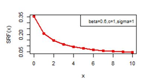
Figure 14 SRF(x) plot for DBD-XII (β, c, γ).
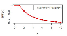
Figure 15 SRF(x) plot for DBD-XII (β, c, γ).
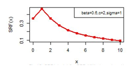
Figure 16 SRF(x) plot for DBD-XII (β, c, γ).
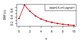
Figure 17 SRF(x) plot for DBD-XII (β, c, γ).
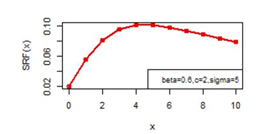
Figure 18 SRF(x) plot for DBD-XII (β, c, γ).
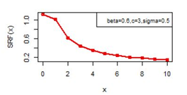
Figure 19 SRF(x) plot for DBD-XII (β, c, γ).
Now,
For checking purpose of moments convergence or divergence, we have
Where
which is convergent if ck-r+1>1 or ck>r
In case of discrete Lomax distribution, for the convergence of moments k should be greater than r. Hence,
for three parameter Burr type XII distribution and discrete Lomax distribution exists if and only if ck>r and k>r respectively. Or in other words when
moments of three parameter Burr type XII distribution exists. There is a one to one correspondence between three parameter continuous Burr type XII distribution and three parameter discrete Burr type XII distribution, as the expressions for survival function, failure rate function, second rate of failure function for DBD-XII
can be directly obtained from continuous Burr type XII distribution by replacing
.
Table 1 and Table 2 exhibits the index of dispersion D = [E(X2) − (E(X))2]/E(X), for different values of the parameters c,
and
for three parameter discrete Burr type XII distribution and discrete Lomax distribution. It can be seen that this variance to mean ratio goes on increasing in case of discrete Lomax distribution as the parameters goes on increasing, and therefore in this case the discrete Lomax distribution seems over dispersed. In case of discrete Burr type XII as
and c goes on increasing the distribution shows under dispersion.
Different Values of γ
|
Different Values of β
|
Parameters |
0.0001 |
0.0003 |
0.0009 |
0.0060 |
0.0200 |
0.0300 |
0.0400 |
0.0500 |
0.10 |
1.0060 |
1.0120 |
1.0250 |
1.1030 |
1.3000 |
1.4610 |
1.6510 |
1.8850 |
0.11 |
1.0060 |
1.0120 |
1.0260 |
1.1060 |
1.3060 |
1.4690 |
1.6630 |
1.8990 |
0.12 |
1.0060 |
1.0120 |
1.0260 |
1.1080 |
1.3120 |
1.4780 |
1.6740 |
1.9140 |
0.14 |
1.0060 |
1.0130 |
1.0280 |
1.1130 |
1.3240 |
1.4950 |
1.6960 |
1.9430 |
0.17 |
1.0070 |
1.0150 |
1.0310 |
1.1210 |
1.3420 |
1.5210 |
1.7310 |
1.9860 |
0.20 |
1.0080 |
1.0160 |
1.0330 |
1.1300 |
1.3610 |
1.5470 |
1.7650 |
2.0300 |
0.25 |
1.0100 |
1.0190 |
1.0380 |
1.1440 |
1.3930 |
1.5900 |
1.8220 |
2.1030 |
0.33 |
1.0120 |
1.0240 |
1.0470 |
1.1680 |
1.4440 |
1.6610 |
1.9140 |
2.2200 |
0.50 |
1.0200 |
1.0360 |
1.0680 |
1.2220 |
1.5550 |
1.8120 |
2.1090 |
2.4680 |
1.00 |
1.0530 |
1.0870 |
1.1450 |
1.3940 |
1.8850 |
2.2550 |
2.6800 |
3.1940 |
1.11 |
1.0620 |
1.1000 |
1.1640 |
1.4330 |
1.9580 |
2.3520 |
2.8060 |
3.3530 |
2.00 |
1.1530 |
1.2220 |
1.3310 |
1.7550 |
2.5520 |
3.1450 |
3.8280 |
4.6530 |
2.50 |
1.2110 |
1.2970 |
1.4310 |
1.9400 |
2.8890 |
3.5940 |
4.4080 |
5.3900 |
3.33 |
1.3140 |
1.4270 |
1.6020 |
2.2520 |
3.4540 |
4.3460 |
5.3760 |
6.6210 |
5.00 |
1.5380 |
1.7060 |
1.9600 |
2.8920 |
4.6040 |
5.8730 |
7.3390 |
9.1120 |
10.00 |
2.2650 |
2.5920 |
3.0810 |
4.8530 |
8.0870 |
10.4860 |
13.2590 |
16.6180 |
Table 1 Index of dispersion for DLomax for different values of
and
Different values of c |
Different values of β |
|
|
|
|
|
|
|
|
Parameters |
0.01 |
0.02 |
0.03 |
0.04 |
0.05 |
0.06 |
0.07 |
0.08 |
0.09 |
|
2 |
0.99 |
0.9945 |
1.0035 |
1.0156 |
1.0307 |
1.0484 |
1.0688 |
1.092 |
1.1181 |
|
3 |
0.9609 |
0.9391 |
0.9222 |
0.9083 |
0.8967 |
0.887 |
0.8789 |
0.8722 |
0.8668 |
|
4 |
0.959 |
0.934 |
0.9131 |
0.8945 |
0.8778 |
0.8624 |
0.8481 |
0.8349 |
0.8225 |
|
5 |
0.9589 |
0.9336 |
0.9121 |
0.8928 |
0.8751 |
0.8584 |
0.8428 |
0.8279 |
0.8137 |
|
6 |
0.9589 |
0.9336 |
0.912 |
0.8926 |
0.8747 |
0.8578 |
0.8419 |
0.8266 |
0.812 |
|
7 |
0.9589 |
0.9336 |
0.912 |
0.8926 |
0.8746 |
0.8578 |
0.8417 |
0.8264 |
0.8117 |
Different values of c |
Different values of β |
|
|
|
|
|
|
|
|
Parameters |
0.11 |
0.12 |
0.13 |
0.14 |
0.15 |
0.16 |
0.17 |
0.18 |
0.19 |
|
2 |
1.1803 |
1.2169 |
1.2579 |
1.3036 |
1.3548 |
1.4122 |
1.4768 |
1.5497 |
1.6324 |
|
3 |
0.8598 |
0.8582 |
0.8577 |
0.8584 |
0.8604 |
0.8636 |
0.8682 |
0.8742 |
0.8816 |
|
4 |
0.8003 |
0.7904 |
0.7811 |
0.7726 |
0.7647 |
0.7576 |
0.7511 |
0.7453 |
0.7403 |
|
5 |
0.7872 |
0.7748 |
0.7628 |
0.7514 |
0.7404 |
0.7299 |
0.7198 |
0.7102 |
0.701 |
|
6 |
0.7843 |
0.7711 |
0.7583 |
0.746 |
0.7339 |
0.7222 |
0.7109 |
0.6998 |
0.6891 |
|
7 |
0.7836 |
0.7703 |
0.7572 |
0.7445 |
0.7322 |
0.7201 |
0.7083 |
0.6967 |
0.6854 |
Different values of c |
Different values of β |
|
|
|
|
|
|
|
|
Parameters |
0.41 |
0.42 |
0.43 |
0.5 |
0.51 |
0.52 |
0.53 |
0.54 |
0.6 |
|
5 |
0.654 |
0.6636 |
0.6756 |
0.848 |
0.8929 |
0.9461 |
1.0094 |
1.0854 |
1.2897 |
|
6 |
0.55 |
0.5504 |
0.5518 |
0.6015 |
0.617 |
0.6356 |
0.6578 |
0.6844 |
0.7539 |
|
7 |
0.5046 |
0.5007 |
0.4973 |
0.4969 |
0.5013 |
0.5074 |
0.5153 |
0.5253 |
0.5531 |
|
8 |
0.4831 |
0.4769 |
0.4711 |
0.4454 |
0.4446 |
0.4447 |
0.4459 |
0.4483 |
0.4577 |
|
9 |
0.4724 |
0.465 |
0.4579 |
0.4181 |
0.4143 |
0.4112 |
0.4088 |
0.4071 |
0.4068 |
|
10 |
0.467 |
0.4589 |
0.451 |
0.4029 |
0.3974 |
0.3923 |
0.3878 |
0.3838 |
0.3777 |
Table 2 Index of dispersion for DBD-XII for different values of β and c when γ=1
Estimation of the parameters of three parameter discrete Burr type XII distribution and discrete Lomax distribution
Estimation of the parameters based on the ML method: Let
be a random sample of size n. If these
are assumed to be iid random variables following three parameter discrete Burr type XII distribution i.e.,
their likelihood function is given by
(5.1)
And (5.1) can be rewritten as follows
(5.2)
where
(5.3)
Taking partial derivatives with respect to
and equating them to zero, we obtain the normal equations.
Which can be solved to obtain the maximum likelihood estimators.
(5.4)
(5.5)
Where
(5.6)
(5.6)
The solution of this system is not possible in a closed form, so by using numerical computation, the solution of the three log-likelihood equations (5.4), (5.5) and (5.6) will provide the MLE of
.
In this study, maximum likelihood estimates of were computed by numerical methods, using the R studio statistical software with the help of “MASS” package. For solving the equations analytically Nelder_Mead optimization method15 is employed.
We here now consider the four possible cases for estimating the parameters.
Case I: known parameters c and γ and unknown parameter β.
yields
Solving the Equation (5.7) analytically gives the maximum likelihood estimator
of the parameter
.
Case II: known parameter c and unknown parameters β and γ.
(5.8)
Solving the Equations (5.7) and (5.8) analytically gives the maximum likelihood estimators β ̂ and γ ̂ of the parameters β and γ.
Case III: known parameter γ and unknown parameters β and c.
yields
(5.9)
Solving the Equations (5.7) and (5.9) analytically gives the maximum likelihood estimators β ̂ and c ̂ of the parameters and .
Case IV: Unknown parameters β , c and γ .
Solving the Equations (5.7), (5.8) and (5.9) analytically gives the maximum likelihood estimators
of the parameters
,
and
respectively.
Estimation of the parameters based on the proportion method: Khan et al.16 proposed and provided a motivation for the method of proportions to estimate the parameters for discrete Weibull distribution. Now, we present a similar method for the three parameter discrete Burr type XII distribution and discrete Lomax distribution for the same reasons as outlined.16 Let
be a random sample from the distribution with pmf (3.1). Define the indicator function by
Denote
by the frequency of the value u in the observed sample.
Therefore, the proportion (relative frequency)
can be used to estimate the probability
. Now we consider the following cases for the purpose of parameter estimation.
Case I: known parameters c and γ and unknown parameter β.
This is the simplest case. The unknown parameter
has a proportion estimator in exact solution, where
(5.10)
denotes the number of zero’s in a sample of size n.
Case II: known parameter c and unknown parameters
and γ.
Let
denote the number of one’s in the sample of size n.
(5.11)
Solving equations (5.10) and (5.11) numerically using Newton_Raphson (N_R) method, gives the proportion estimators
and
of the parameters
and
.
Case III: known parameter γ and unknown parameters
and c.
Solving equations (5.10) and (5.11) numerically using Newton_Raphson (N_R) method, gives the proportion estimators
and
of the parameters
and
.
Let
denote the number of two’s in the sample of size n.
(5.12)
Solving the Equations (5.10), (5.11) and (5.12) analytically using Newton_Raphson (N_R) method, gives the proportion estimators
of the parameters
respectively.
Some theorems related to three parameter discrete Burr type XII distribution and discrete Lomax distribution
In this section we discuss some important theorems which relate three parameter discrete Burr type XII Distribution and discrete Lomax distribution with some important discrete class of continuous distributions already in the literature.
Theorem 1: Let X be random variable following three parameter continuous Burr XII distribution with
Then
where
Proof: Proof is straight forward, since
, so clearly if
Then
.
Theorem 2: If
then
follows discrete inverse Weibull distribution i.e., DIW (
)
Proof:-
Which is the survival function of a discrete inverse Weibull distribution.
Hence
Theorem3: If
then
follows discrete Raleigh distribution i.e., DRel
Proof:-
which is the survival function of a discrete Raleigh distribution.
Hence
.
Corollary. If
then
Application of discrete Lomax distribution and three parameter discrete Burr type XII distribution in medical science
Here we consider the data set of counts of cysts of kidneys using steroids as given in the Table 3. The example data set originated from a study1 investigating the effect of a corticosteroid on cyst formation in mice fetuses undertaken within the Department of Nephro-Urology at the Institute of Child Health of University College London. Embryonic mouse kidneys were cultured, and a random sample was subjected to steroids (110). Table 4 exhibits some descriptive measures of count data of cysts of kidneys using steroids based on 1000 bootstrap samples.
For the purpose of parameter estimation, we employ the fitdistr procedure in R studio statistical software to find out the estimates of the parameters. The ML estimates and their standard errors provided by the fitdistr procedure are given in the Table 5. In Figure 20 the empirical cdf of the number of cysts in a kidney using steroid has been shown.
We compute the expected frequencies for fitting discrete Lomax, three parameter discrete Burr type XII, Poisson, Geometric, Inflated Poisson and DRayleigh distributions with the help of R studio statistical software and Pearson’s chi-square test is applied to check the goodness of fit of the models discussed. The calculated figures are given in the Table 5.
The p-values of Pearson’s Chi-square statistic are 0.532, 0.352, 0.0008, 0.000, 0.000 and 0.0006 for three parameter discrete Burr type XII, discrete Lomax, Zero Inflated Poisson, Poisson, Discrete Raleigh and geometric distributions, respectively Table 6. This reveals that Zero Inflated Poisson, Poisson, Geometric and discrete Rayleigh distributions are not good fit at all, whereas three parameter Burr type XII distribution and two parameter discrete Lomax distributions are good fit distributions with three parameter discrete Burr type XII model being the best one. The null hypothesis that data come from three parameter Burr type XII and two parameter discrete Lomax distributions is accepted. Figure 21 exhibits the graphical overview of the fitted distributions.
We have compared three parameter discrete Burr type XII distribution and two parameter discrete Lomax distribution with discrete Raleigh, Poisson, Zero Inflated Poisson and Geometric distributions using the Akaike information criterion (AIC), given by Akaike17 and the Bayesian information criterion (BIC), given by Schwarz.18 Generic function calculating Akaike's ‘An Information Criterion’ for one or several fitted model objects for which a log-likelihood value can be obtained, according to the formula -2*log-likelihood + k*npar, where npar represents the number of parameters in the fitted model, and k = 2 for the usual AIC, or k = log(n) (n being the number of observations) for the so called BIC or SBC (Schwarz's Bayesian criterion).
From Table 7, it is obvious that AIC and BIC criterion favors three parameter discrete Burr type XII and two parameter Lomax distributions in comparison with the Poisson, Zero Inflated Poisson, discrete Raleigh and Geometric distributions, in the case of Counts of cysts of kidneys using steroids.
Figure 21 exhibits graphical overview of the AIC, BIC and negative loglikelihood values for fitted distributions.
|
Counts of cysts of kidneys using steroids
|
0
|
1
|
2
|
3
|
4
|
5
|
6
|
7
|
8
|
9
|
10
|
11
|
Total
|
|
Frequency
|
65
|
14
|
10
|
6
|
4
|
2
|
2
|
2
|
1
|
1
|
1
|
2
|
110
|
Table 3 Counts of cysts of kidneys using steroids
Descriptive Measures |
Statistic |
Standard Error |
Bootstrapa |
Bias |
Standard Error |
95% Confidence Interval |
Lower |
Upper |
Sum |
153 |
|
|
|
|
|
Mean |
1.39 |
0.236 |
0.01 |
0.23 |
0.95 |
1.87 |
Standard Deviation |
2.472 |
|
-0.018 |
0.309 |
1.812 |
3.053 |
Variance |
6.112 |
|
0.009 |
1.511 |
3.283 |
9.324 |
Skewness |
2.293 |
0.23 |
-0.04 |
0.308 |
1.685 |
2.908 |
Kurtosis |
5.089 |
0.457 |
-0.069 |
1.911 |
1.963 |
9.531 |
Valid N (listwise) |
N |
110 |
|
0 |
0 |
110 |
110 |
a. Bootstrap results are based on 1000 bootstrap samples |
Table 4 Descriptive statistics of Counts of cysts of kidneys using steroids
Distribution |
Parameter Estimates |
Standard Error of the Estimates |
Model Function |
Discrete Lomax |
|
[0.098, 0.953] |
where
|
Poisson |
|
[0.112] |
|
DRayleigh |
q=0.90 |
[0.009] |
|
Geom |
q=0.418 |
[0.03] |
|
Three Parameter Burr type XII |
|
[0.002, 0.087, 5.06] |
where
|
Zero Inflated Poisson |
|
[0.049, 0.283] |
|
Table 5 Estimated parameters by ML method for fitted distributions
X |
Observed |
DBD-XII |
Discrete Lomax |
ZIP |
Poisson |
Discrete Raleigh |
Geometric |
0 |
65 |
63.32 |
61.89 |
64.92 |
27.4 |
11 |
45.98 |
1 |
14 |
18.19 |
21.01 |
5.82 |
38.08 |
26.83 |
26.76 |
2 |
10 |
9.29 |
9.65 |
9.52 |
26.47 |
29.55 |
15.57 |
3 |
6 |
5.49 |
5.24 |
10.38 |
12.26 |
22.23 |
9.06 |
4 |
4 |
3.52 |
3.17 |
8.48 |
4.26 |
12.49 |
5.28 |
5 |
2 |
2.39 |
2.06 |
5.55 |
1.18 |
5.42 |
3.07 |
6 |
2 |
1.69 |
1.42 |
3.02 |
0.27 |
1.85 |
1.79 |
7 |
2 |
1.23 |
1.02 |
1.41 |
0.05 |
0.5 |
1.04 |
8 |
1 |
0.92 |
0.76 |
0.58 |
0.01 |
0.11 |
0.61 |
9 |
1 |
0.7 |
0.58 |
0.21 |
0 |
0.02 |
0.35 |
10 |
1 |
0.55 |
0.46 |
0.07 |
0 |
0 |
0.21 |
11 |
2 |
2.71 |
2.73 |
0.03 |
0 |
0 |
0.29 |
P-Values |
0.532 |
0.352 |
0.0008 |
0.000 |
0.000 |
0.0006 |
Table 6 Table for goodness of fit
Criterion |
Discrete Lomax |
DBD-XII |
ZIP |
Poisson |
Discrete Raleigh |
Geometric |
Neg-Loglike |
170.4806 |
168.7708 |
182.2449 |
246.21 |
277.778 |
178.7667 |
AIC |
344.9612 |
343.5415 |
368.4897 |
494.42 |
557.556 |
359.5333 |
BIC |
350.3622 |
351.6429 |
373.8907 |
497.1205 |
560.2565 |
362.2338 |
Table 7 AIC, BIC and Negative loglikelihood values for fitted distributions
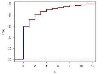
Figure 20 ECD of Counts of cysts of kidneys using steroids.
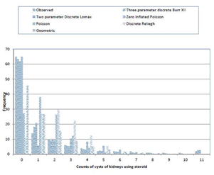
Figure 21 Overview of fitted distributions.
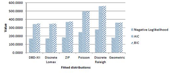
Figure 22 AIC, BIC and Negative loglikelihood values for fitted distributions.
Acknowledgments
We don’t have any funding source. In acknowledge, mention, author is thankful reviewers for their construct and valid review which brought the quality of the manuscript up.
Conflicts of interest
References
- Chan S, Riley PR, Price KL, et al. Corticosteroid-induced kidney dysmorphogenesis is associated with deregulated expression of known cystogenic molecules, as well as indian hedgehog. American Journal of Physiology-Renal Physiology. 2009;298(2):346–356.
- McElduff F, Cortina Borja M, Chan S, et al. When t-tests or Wilcoxon-Mann-Whitney tests won't do. Advances in Physiology Education. 2010;34(3):128–133.
- Kapur KC, Lamberson LR. Reliability in Engineering Design. John Wiley & Sons, New York, USA. 1997.
- JF Lawless. Statistical models and methods for lifetime data. Canadian Journal of Statistics 1982;10(4):316–317.
- Sinha Sk. Reliability and Life testing. Wiley Eastern Ltd, New Delhi. 1986.
- Roy D. The Discrete Normal Distribution. Communications in Statistics-Theory and Methods. 2003;32(10):1871–1883.
- Roy D. Discrete Rayleigh Distribution. IEEE Transactions on Reliabil. 2004;53(2):255–260.
- Krishna H, Singh Pundir P. Discrete Burr and discrete Pareto distributions. Statistical Methodology. 2009;6(2):177–188.
- Jazi MA, Lai C, Alamatsaz MH. A discrete inverse Weibull distribution and estimation of its parameters. Statistical Methodology. 2010;7(2):121–132.
- Para BA, Jan TR. Discretization of Burr-Type III Distribution. Journal of Reliability and Statistical Studies. 2014;7(2):87–94.
- Gómez Déniz E, Calderín Ojeda E. The discrete Lindley distribution: properties and applications. Journal of Statistical Computation and Simulation. 2011;81(11):1405–1416.
- Nekoukhou V, Alamatsaz MH, Bidram H. A Discrete Analog of the Generalized Exponential Distribution. Communications in Statistics-Theory and Methods. 2012;41(11):2000–2013.
- Burr IW. Cumulative Frequency Functions. Ann Math Statist. 1942;13(2):215–232.
- Roy D. Reliability Measures in the Discrete Bivariate Set-Up and Related Characterization Results for a Bivariate Geometric Distribution. Journal of Multivariate Analysis. 1993;46(2):362–373.
- Nelder JA, Mead R. A simplex method for function minimization. The Computer Journal. 1969;7(4):308–313.
- Khan MSA, Khalique A, Abouammoh AM. On estimating parameters in a discrete Weibull distribution. IEEE Transactions on Reliabil. 1989;38(3):348–350.
- Akaike H. A new look at the statistical model identification. IEEE Transactions on Automati. 1974;19(6):716–723.
- Schwarz G. Estimating the Dimension of a Model. Ann Statist. 1978;6(2):461–464.

©2016 Para, et al. This is an open access article distributed under the terms of the,
which
permits unrestricted use, distribution, and build upon your work non-commercially.


