Rolling variance atlas is proved to be very useful in identifying boundaries and data patterns in this study, but faces a vulnerable problem of background noise in the actual dataset. Luckily, The Kolmogorov–Zurbenko Adaptive, KZA algorithm is available to deal with abrupt changes or discontinuities in the presence of heavy background noise. Two–dimensional simulated samples are generated to demonstrate signal recoveries and their boundary identification by mean of KZA algorithm and rolling variance atlas. Simulation investigation showed that rolling variance atlas could identify boundaries resulted from signal discontinuities, even when background noise is stronger than signal discrepancy.

Keywords: rolling variance atlas, boundary identification, KZA algorithm, non–parametric, two–dimensional data

Understanding the impact of spatial patterns and processing features on health is a key element in public health and epidemiology fields.^1–3 These patterns characterized on a two or higher dimensional settings, are usually forming visible and/or invisible boundaries between various types of pattern attributes (color, texture, intensity, etc.).^4–6 Therefore, boundary detection constitutes a crucial initial step before performing downstream tasks such as pattern characterization and feature interpretation.

A boundary is a significant local change in the pattern attribute(s), usually associated with a discontinuity in either the pattern attribute or the first derivative of the pattern attribute.⁷ Zurbenko and his students used local variance (sample variance) to visualize discontinuities (data breaks) in their previous ‘Comprehensive Aerological Reference Data’ project.⁸ In time series analysis, a common technique to assess the parameters’ stability is to compute their estimates over a rolling window through the study period.⁹ If the parameters are stable, then the estimates over the rolling windows should be similar; if the parameters change significantly at some point, then the rolling estimates should capture this substantial variation. For example, Aslan applied bootstrap rolling window estimation to display the existence of inverted U–shaped economic growth in the US during 1982–2013;¹⁰ Comin and colleagues applied rolling window estimates in their endogenous growth model to explain the evolution of the first and second moments of productivity growth at the aggregate and firm level.¹¹ However, all these approaches are limited to one dimensional settings. In this paper, we propose a new approach to apply rolling variance at two–dimension level to identify and locate boundaries of interest.

Considering the robustness and generality of the approach, assume that n observations were observed on a 2D space. These observations from two larger objects connected to each other, and one smaller object stays away from the larger ones (Figure 1). To sense the overall spatial variations, the sample variance (1) is often used to characterize the spatial variation:

V =$\frac{1}{n-1}{\displaystyle \sum _{i=1}^n{(O_i-m)}^2}$ (1)

where O_i is i^th observation and m is the mean of the n observations.

However, the sample variance is substantially biased if the observations comprise clusters, which usually result in patterns as shown in Figure 1. In such case for a temporal series of data, Blue⁴ recommended calculating the moving variance to reduce the bias. Similarly, instead of the moving variance of a temporal series, a series of variances are calculated for observations over the local area respectively, then form a spatial variance atlas (Figure 1C & D).

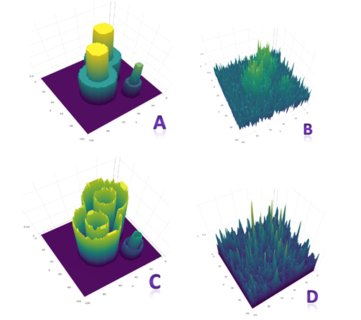
Figure 1 The visualization of simulated spatial data and rolling variance atlas: A. Object signals (max=1.5) on a 2D space; B. the same signals were embedded in noise (σ=0.3, 20% of signal maximum); C. rolling variance atlas (window size=16) of signals in A; D. rolling variance atlas for data in B.

The rolling variance

The rolling sample variances, or rolling variances, are calculated based on a dynamic spatial window. Given that this spatial window is moving, when its size is optimal, the significant local changes will be captured. It is neither necessary to make any assumption, nor to model anything, so it is a nonparametric statistic. However, very often actual data might be embedded in heavy background noises,⁸ direct application of rolling variance to real data could fail to identify the significant local variations, or recognize false variations (Figure 1D). Fortunately, the Kolmogorov–Zurbenko Adaptive, KZA package provides algorithms to examine abrupt changes in the presence of heavy background noise.^12–15 It is reasonable to apply KZA algorithms to actual data first, before rolling variance analysis for boundary identification performed.

Spatial rolling window

The spatial rolling variance utilizes the spatial information, to help decide the size and constituents of a rolling window (Figure 2). Given that there exists an observation ‘v/(i, j)’, we first assign the coordinates for all the observations around: [(i±d), (j±d)], d=1, 2, 3…, we could design rolling windows with any size, such as an arbitrary rolling window with d=1, which covers the area labeled with ‘v’ (Figure 2), containing n_r=9 observations. Then we can calculate its rolling mean m_r in (2) and rolling variance v_r in (3).

Figure 2 Spatial rolling window design.

The rolling variances v_r, calculated based on windows located at certain spatial area, form a spatial variance atlas, which can quantitatively evidence the significant local changes.

Rolling variance atlas, a practical boundary indicator

Assuming that we observed ‘8–o’ shaped signals on a 2D space (Figure 3). We calculated their rolling variance atlas with rolling windows similar to those mentioned in 2.2; For example, when d=1 the window size equals (1+2d)2=9, the area labeled with ‘V’ in Figure 2; when d=2 the window size equals 25, and so on; see Table 1 for details.

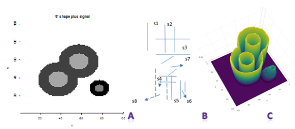
Figure 3 Clustering patterns of the observed signals (A) and rolling variance atlas generated with rolling window size 36 (B) and 49 (C). s1, s2, s3, s4, s5, s6, s7 and s8 are the corresponding distance between adjacent boundaries.

In theory, the rolling variance atlas can perfectly reflect the local variations (including boundaries), once optimal rolling windows are applied (Figure 1C). As long as the side lengths of rolling windows are smaller than the distance between the adjacent boundaries of interest, e.g. 2d+1 is smaller than the minimum of s1 through s8 (Figure 3A), rolling variance atlas can successfully display the boundaries. When the window side length equals the distance between adjacent boundaries, the rolling variance atlas starts to be overlapped (see the small object in Figure 3B); as the window side length continues to grow, the rolling variance atlas fails to identify the existing boundary (see the small object in Figure 1C & Figure 3C).

When resolution permits, it is always possible to find an optimal window size under limited background noises. It is obvious that noise is a big concern for real data (Figure 1B &1D). Therefore, it depends on efficient removal of background noise for rolling variance atlas to identify boundaries of interest (Figure 4).

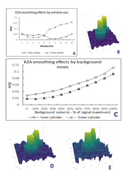
Figure 4 Illustration of KZA smoothing effects by window size (A) and background noise (B through E). B. noise – N(µ=0, σ=0.375, 25% of signal maximum); D. noise – N(µ=0, σ=0.75, 50% of signal maximum); E. noise – N(µ=0, σ=1.2, 80% of signal maximum).

Rolling variance atlas and influence of background noise

As mentioned above, background noise dramatically interferes with rolling variance atlas. To better address this issue, assume that we have simulated data (Figure 5A), this data is embedded in noises (Figure 5B), as we usually face in our life. Without copying with the noises embedded in the data, rolling variance can go nowhere of boundary identification. Luckily KZA(m,k) algorithm is available to be implemented to powerfully ‘suppress’ the noise without distorting other existed patterns of the data.16-19 To illustrate the effect of KZA algorithm, we introduce: mean M in (4), variance V in (5), mean squared error MSE in (5) and error indicator EI in (6). EI will be used to evaluate how background noise affects KZA’s filtration and rolling variance atlas.

M =$\frac{1}{N}{\displaystyle \sum }_{i,j}v\$KZ{A}_{i,j}$ (4)

V =$\frac{{{\displaystyle \sum }}_{i,j}{\left|v\$KZ{A}_{i,j}-M\right|}^2}{N-1}$ (5)

MSE = $\frac{1}{N}{\displaystyle \sum }_{i,j}{\left|Signa{l}_{i,j}-v\$KZ{A}_{i,j}\right|}^2$ (6)

EI = $\sqrt{\frac{MSE}{V}}$ (7)

here, i, j are the signal coordinate index on the sample space, $v\$KZA$ smoothed signal with KZA algorithm, N, is the signal sample size.

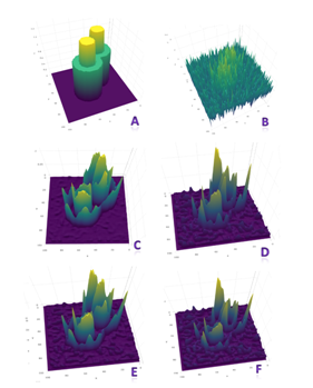
Figure 5 Illustration of rolling variance atlas of signals embedded in various levels of background noises: A. signals; B. signals embedded in noise with σ =0.75, 50% of signal maximum; C. KZA reconstructed signals embedded in noise with σ =0.375, 25% of signal maximum; D. KZA reconstructed signals embedded in noise with σ =0.75, 50% of signal maximum; E. KZA reconstructed signals embedded in noise with σ =1.2, 80% of signal maximum; F. KZA reconstructed signals embedded in noise with σ = 1.35, 90% of signal maximum.

Before started looking at the background noise’s interference with KZA, we need to figure out the optimal smoothing window size for KZA to apply in this experiment. Assumed that there were simulated signal data–a couple of stacked cylinders attached to each other at the bottom part (Figure 5A); this signal data was embedded in the background noise (Figure 5B). Smoothing effects of KZA algorithm by window size are displayed in Figure 4A. Figure 4B shows the reconstructed signals by using window size of 9. After we applied KZA algorithm to the simulated data, influence of noise on KZA’s smoothing performance is summarized in Figure 4C. Although signal reconstruction (both the inner and outer cylinders) is interfered by background noise obviously, KZA algorithm could copy with noise in a decent shape, with noise σ reaches up to 80% of the signal maximum (Figure 4D, 4E). We also addressed this in detail in our previous study.20,21

KZA algorithm made it possible for rolling variance calculation for signals embedded in heavy background noise (Figure 5). Overall, rolling variance atlas could identify signal boundaries embedded in noises with noise σ up to 50% of signal maximum (Figure 5D); when the noise σ goes up to 80% of signal maximum, rolling variance atlas could barely identify the boundaries (Figure 5E), but as σ reaches 90% of signal maximum, it cannot successfully identify the entire boundary patterns (Figure 5F), although it could still identify part of the boundaries, such as the inner cylinder boundaries.

Influence of signal discrepancy forming the boundaries on rolling variance

Boundary is formed due to signal discontinuity and/or significant local changes. In this section, we try to investigate how much a local change is enough for rolling variance to detect it. To focus on our target, we would use a simpler simulated signal data (Figure 6A), with the inner cylinder = 1.5 and outer cylinder = 0.75; and let this signal to be embedded in the background noise with a distribution of N(µ = 0, σ = 0.375, 25% of signal maximum). We fix the inner cylinder while gradually increase outer cylinder from 0.75 to 1.5, such that the percentage of relative signal discrepancy (RSD): 100*(inner–outer)/outer would drop from 100% to 0.

To calculate rolling variance, we had to reconstruct the actual signal from the background noise. Using an appropriate smoothing window, KZA algorithm could successfully reconstruct the signal (Figure 6B). EI indicator for inner cylinder did not affect by signal discrepancy change, while the EI for outer cylinder gradually increased parallel to signal discrepancy change; it makes sense because inner cylinder was fixed. After signal is reconstructed, rolling variance could be calculated (Figure 6C–6F). Rolling variance could always detect the outer cylinder boundary; However, rolling variance could only be able to identify the inner cylinder boundary as the relative signal discrepancy level was not lower than 25% (Figure 6E), where the absolute signal difference = 0.3. This local difference/change was smaller than background noise. When RSD dropped to 18% (Figure 6F), rolling variance could barely identify the inner boundary.

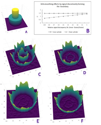
Figure 6Illustration of KZA smoothing effects and rolling variance atlas by signal discrepancy. A. Signals only; B. KZA smoothing effects by signal discrepancy; C. rolling atlas (RSD=0); D. rolling atlas (RSD=54%); E. rolling atlas (RSD=25%); F. rolling atlas (RSD=18%).

Influence of distance between adjacent boundaries on rolling variance atlas

As we learned in section 2, rolling variance relies solely on the removal of background noise; and KZA algorithm has been proved to be an adept in removing background noise without twisting the data structures. However, KZA software does require that signals under smoothing are distinguishable.20 We will investigate how far away is enough for adjacent boundaries to be distinguished / detected by rolling variance atlas. Provided that within a background noise (σ = 25% of signal maximum), there are embedded “8–shape” cylinder signals on a 100x100 sample space, their centers are located at (38, 38) and (58, 58) respectively (top, Figure 7B). The diameters for inner cylinders are 18, and 38 for outer cylinders, such that a = 10.28 and b = 28.28 (Table 2). To investigate the influence of distance between the inner cylinders (a) on the performance of rolling variance, let one set of cylinders move towards another set of cylinders, with step = ∆d. Table 2 shows the distance between the centers of two sets of cylinders (b) and distance between the inner cylinders (a), while one set of cylinders moving towards another set of cylinders.

KZA smoothing effects by selected distance ‘a’ are showed in Figure 7A. The error indicator EI for inner cylinders was gradually increasing as the inner cylinders got closer and closer. Rolling variance was capable of distinguishing the inner boundaries until ∆d = 6 (Figure 7D), where distance a = 1.8. When ∆d = 7 and distance a = 0.38, rolling variance could not distinguish the boundaries of the inner cylinders, where the boundaries are mingled to each other (Figure 7E). This indicates that rolling variance performs very well in identifying boundaries once the background noises are taken care of.

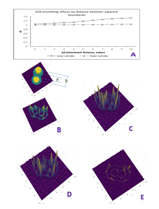
Figure 7Illustration of KZA smoothing effects and rolling variance atlas by signal boundary distance. A. KZA smoothing effects by selected boundary distance; B. Signals (top) and rolling variance atlas with ∆d=3 (bottom); C. Rolling variance atlas with ∆d=5; D. Rolling variance atlas with ∆d=6; E. Rolling variance atlas with ∆d=7.

In identifying boundaries with rolling variance, background noise is its Achilles' heel. Fortunately, KZA algorithm is available for us to reconstruct actual data from heavy background noise without smoothing out data properties. This article is trying to convince readers: (1). Rolling variance atlas is useful in identification of boundaries and data patterns. (2). Rolling variance atlas is simple; it does not require any specific assumptions of your data. (3). With the aids of KZA algorithm, rolling variance atlas can handle data embedded in heavy noise; it can apply to data in various of format, such as one–dimensional data vector, two–dimensional data matrix, three–dimensional data array, and even higher dimensional data (with modification). Rolling variance atlas would even work better while applied to higher–dimensional data, since KZA algorithm works better under high–dimensional settings.

None.

Author declares that there is no conflict of interest.

1. Michael Jerrett, Sara Gale, Caitlin Kontgis. Spatial Modeling in Environmental and Public Health Research. Int J Environ Res Public Health. 2010;7(4):1302–1329.
2. Amy H Auchincloss, Samson Y Gebreab, Christina Mair, et al. A Review of Spatial Methods in Epidemiology, 2000–2010. Annu Rev Public Health. 2012;(33):107–122.
3. Sherman RL, Henry KA, Tannenbaum SL, et al. Applying Spatial Analysis Tools in Public Health: An Example Using SaTScan to Detect Geographic Targets for Colorectal Cancer Screening Interventions. Prev Chronic Dis. 2014;11:130264.
4. Jakey Blue, Argon Chen. Spatial Variance Spectrum Analysis and Its Application to Unsupervised Detection of Systematic Wafer Spatial Variations. IEEE Transactions on Automation Science and Engineering. 2011;8(1):56–66.
5. Wei–Ying Ma, BS Manjunath. Edge Flow: a technique for boundary detection and image segmentation. IEEE Transactions on Image Processing. 2000;9(8):1375–1388.
6. KV Subbarao, FJ Ferrandino, JJ Hao. Spatial Analysis Based on Variance of Moving Window Averages. Journal of Phytopathology. 2006;154(6):349–360.
7. ER Davies. Machine Vision. 2nd ed. In: A volume in Signal Processing and its Applications. 2005; p. 131–157.
8. Zurbenko IG, Porter PS, Gui R, et al. Detecting Discontinuities in Time Series of Upper–Air Data: Development and Demonstration of an Adaptive Filter Technique. AMS. 196;(9):3548–3560.
9. Eric Zivot, Jiahui Wang. Rolling Analysis of Time Series. Modeling Financial Time Series with S–PLUS®. New York: Springer;2006.
10. Aslan A, Destek MA, Okumus I. Bootstrap rolling window estimation approach to analysis of the Environment Kuznets Curve hypothesis: evidence from the USA. Environ Sci Pollut Res Int. 2018;25(3):2402–2408.
11. Diego Comin, Sunil Mulani. A theory of growth and volatility at the aggregate and firm level. Journal of Monetary Economics. 2009;56:1023–1042.
12. B. Close, I Zurbenko. Kolmogorov–Zurbenko adaptive filters.  KZA. 2016.
13. Igor G. Zurbenko, Devin Smith. Kolmogorov–Zurbenko filters in spatiotemporal analysis. WIREs in Computational Statistics. 2017;10(1).
14. Kolmogorov–Zurbenko Filters. Wikipedia.
15. W Yang, I Zurbenko. Kolmogorov–Zurbenko filters. WIREs in Computational Statistics. 2010;(2):340–351.
16. Zurbenko IG, Porter PS, Gui R, et al. Detecting Discontinuities in Time Series of Upper–Air Data: Development and Demonstration of an Adaptive Filter Technique. Journal of Climate. 1996;(9):3548–3560.
17. Zurbenko IG, Cyr DD. Climate fluctuations in time and space. Climate Research. 2013;57:93–94.
18. Zurbenko I, Luo M. Surface Humidity Changes in Different Temporal Scales. American Journal of Climate Change. 2015;4:226–238.
19. Valachovic E, Zurbenko I. Multivariate Analysis of Spatial–Temporal Scales in Melanoma Prevalence. Cancer Causes Control. 2017;28(7):733–743.
20. Igor G Zurbenko, Mingzeng Sun. Applying Kolmogorov–Zurbenko Adaptive R–Software. International Journal of Statistics and Probability. 2017;6(5):110–118.
21. I Zurbenko, Ming Luo. Restoration of Time–Spatial Scales in Global Temperature Data. American Journal of Climate Change. 2012;1(3):154–163.