Bayesian estimation approaches can accommodate a variety of latent-variable models including structural equation modeling (SEM). Despite their theoretical appeal, it can be non-trivial to implement appropriate estimation algorithms in these contexts. There is a strong need of detailed explanations of the impact of the various estimation options on how a MCMC sampler behave to empower users of Bayesian estimation methods to understand choices made by programs and, perhaps, to make them aware of challenges in developing their own MCMC estimation procedure. In this paper, a Markov chain Monte Carlo (MCMC) estimation method is illustrated using a one-factor model and a two-factor model with a directional path. The objective is to illustrate in an accessible manner how different estimation choices such as the choice of starting values, the choice of jump sizes for the proposal distribution, and the choice of model complexity impact MCMC estimation results.

Keywords: structural equation modeling, markov chain monte carlo, parameter estimation, bayesian inference, metropolis algorithm

Structural equation modeling (SEM; Bollen,¹) is a key latent-variable modeling framework in the social and behavioral sciences. It is generally used for understanding how observable indicators relate to latent variables that are postulated to represent unobservable constructs and how these latent variables influence each other. SEM can accommodate a variety of research questions including those that lead to multi-group estimation, multi-level estimation, missing data estimation, and longitudinal estimation, both in isolation and in combination.

Mathematically, the aim of SEM is to test the hypothesis that the observed covariance matrix for a set of observable indicator variables in the population,$\Sigma$ , is equal to the covariance matrix that is implied by the particular SEM that is fitted to population data,$\Sigma \left(\theta \right)$ . Since population data are generally not available to researchers, this hypothesis is tested by comparing the fit of a model-implied covariance matrix to the covariance matrix computed based on sample data, S. In the notation $\Sigma \left(\theta \right)$ ,$\theta$ denotes a joint vector of different types of model parameters, which typically include (a) loadings of observable indicator variables on the latent variables, (b) error variances associated with the observable indicator variables, (c) variances of the latent variables themselves, (d) correlations or regression coefficients between latent variables, and (e) means of latent variables. As we shall see below for the models used in this paper, all of these parameters, except for latent means, need to be estimated.

In order to assess whether the model-implied covariance matrix reproduces the observed-data matrix reasonably well, different fit functions or target functions need to be specified, whose definition depends on the estimation approach used. Common estimation approaches include maximum likelihood (ML) estimation (Bollen,¹), generalized least square (GLS) estimation (Browne,²), and weighted least squares (WLS) estimation (Browne,³). All three estimation approaches provide consistent, efficient, and unbiased parameter estimates and asymptotic standard errors if their respective assumptions (e.g., adequate sample size, appropriate distributional forms of indicator and latent variables, and properly specified model structure) are met along with an omnibus test of model fit (Bollen,¹ for more details of these fit functions).

Even though these estimation methods have been widely used, they can be challenging to implement when the parametric complexity of a specified SEM model is high. This is the case, for example, when SEM models are fit to ordinal indicator variables, when mixture distributions are include in an SEM model, or when a multi-level SEM model is estimated. Consequently, these situations are one primary motivation for looking at alternative estimation approaches. The predominantly used alternative approach is a Bayesian estimation approach (e.g., Gelman;⁴ Lee;⁵ Choi & Levy;⁶ Levy & Mislevy,⁷), which is the focus of this paper.

In Bayesian estimation approaches, point estimates of parameters their corresponding interval estimates are estimated from what is known as the posterior distribution of each parameter, which is also known as the marginal density of each parameter. It is a function of prior information about the parameter values, often provided by experts or assumed to be diffuse, and information about the parameter values contained in the data. Both types of information can be modeled using specific distributions. Specifically, the posterior distribution for each parameter is proportional to the product of the prior distribution and the likelihood, which means that posterior information about a model parameter is a statistical compromise between prior information and information contained in response data.

Despite this relatively straightforward conceptual notion, it is often impossible to analytically derive the exact form of the posterior distribution of each parameter, especially for complex models such as SEM models. Thus, one requires a mechanism for obtaining a numerical approximation of the posterior distribution, which is accomplished by sampling from it. Yet, sampling from the posterior distribution is also a challenging task because the posterior distribution of interest is usually a complex density function composed of several individual distribution functions for different parameter sets.

In recent years, Markov chain Monte Carlo (MCMC) estimation has been refined for this purpose and it is currently the methodological state-of-the-art for estimating various latent variable models. In a nutshell, a “Markov chain” is a statistical process that produces future outcomes that are independent of past outcomes, which enable us to sample each parameter as if they were independent each other although they were from a complex joint density. The term “Monte Carlo” essentially refers to the fact that sampling is done in a random, albeit structurally systematic, fashion. There exist a wide variety of different sampling algorithms under this heading, which have been designed to function optimally for different data structures (e.g., Junker,⁸ for an overview).

Even though numerous rigorous treatments of MCMC estimation exist in the literature (e.g., Lee;⁵ Chen, Choi, Stapleton, and Weiss,⁹ or Choi and Levy,⁶ in the context of SEM), there is a large gap between these theoretical treaties and practical implementations of it, which can be far from trivial. Most practically-oriented overview articles on Bayesian estimation (e.g., Kim and Bolt¹⁰ in the context of item response theory models, or Lynch¹¹ for statistical models more generally) use very simple data sets and do not discuss the intricacies of actually implementing MCMC estimation for a specific model. Fortunately, there are programs available that handle some MCMC estimation choices automatically such as BUGS (Spiegelhalter, Thomas, Best, & Gilks,¹²) or AMOS 7.0 (Arbuckle,¹³).

Although the technical advantages of MCMC over traditional estimation approaches (e.g., ML estimation) have been advocated for, the details of MCMC estimation method for SEM are typically not widely understood among both methodologists and applied researchers working with SEM models. This is, in part, due to a lack of detailed illustrations of how to actually implement MCMC algorithms beyond merely asking a particular software program to estimate an SEM model. That is, even though programs such as BUGS or AMOS 7.0 make estimation more practically convenient, their availability alone has not helped users to understand how they function at a deeper level “behind the scenes”.

The purpose of this paper is to provide an accessible illustration of how different estimation choices impact how a MCMC sampler behave to empower users of Bayesian estimation methods to understand choices made by programs and, perhaps, to make them aware of challenges in developing their own MCMC estimation procedure. The objective is to illustrate a MCMC algorithm behavior and not to provide a comprehensive review of various types of MCMC algorithms. Thus, two simple SEM models and one simple MCMC sampler will be used under a variety of estimation conditions, which are (a) different choices of starting values for model parameters, (b) different choices of jump sizes for the proposal distribution in the sampler, and (c) different levels of complexity of the SEM models. Specifically, the Metropolis algorithm (Metropolis & Ulam;¹⁴ Metropolis, Rosenbluth, Rosenbluth, Teller & Teller,¹⁵) is utilized to estimate a one-factor model, which is akin to a confirmatory factor analysis model, and a two-factor model with a directional path between the latent variables under these different conditions.

Traditional estimation approaches such as ML, GLS, and WLS involve optimization routines that employ the first- and/or second-order partial derivatives of the target function, which makes them gradient-based search algorithms (Lee;⁵ Jöreskog,¹⁶). Such algorithms include, for example, the Newton-Raphson or the Gauss-Newton method type algorithms (Kennedy & Gentle,¹⁷). For a detailed description of general gradient-based search algorithms, we recommend, for example, Süli and Mayers¹⁸ and for a detailed descritpion gradient-based search algorithms within an SEM context we recommend, for example, Lee.⁵

For the purposes of this paper, suffice it to say that independent of which optimization algorithm is employed, the basic idea of different algorithms is the same. Using the first- and/or second-order partial derivatives, these algorithms iteratively search the parameter space of the target function to determine its minimum or maximum, depending on how the target function is defined. The maxima (or minima) found upon convergence are the ML estimates of the parameters, and their standard errors can be computed using the inverse of the Hessian matrix, which is the matrix of second-order partial derivatives.

Challenges in gradient-based estimation methods

Determining parameter estimates using gradient-based estimation is, metaphorically speaking, akin to mountain climbing such that the goal is to find the highest mountaintop among all of the mountains in a particular range. The biggest challenge is that there might be multiple mountaintops that one could aim for (i.e., multiple local maxima exist), and that the mountaintop that one ends up climbing depends on where one starts the climb as some mountaintops are hidden from one’s view at a particular location (i.e., the global maximum might not be reached).

As the sample size decreases, the problem of finding local, rather than global, maxima tends to get worse. Furthermore, these estimation algorithms might not even converge to any solution when sample sizes are small (e.g., less than 100 observations) and/or when models become very complex (Browne;³ Choi, et al.,¹⁹ Choi, et al.,²⁰).

Advantages of MCMC estimation methods

MCMC estimation methods, which are simulation-based estimation methods, provide a powerful, albeit not perfect, solution to these problems. Nevertheless, MCMC estimation provides a virtually universal tool to deal with optimization problems generally (Andrieu, et al.,²¹ Dyer, et al.,²² Jerrum & Sinclair,²³). MCMC estimation approaches also have been shown to provide methodological advantages in SEM specifically. For example, they can yield reliable parameter estimates even with small sample sizes, they can flexibly accommodate data missing by design or at random, and they can handle non-linear, mixture, or hierarchical models (e.g., Arminger, & Muthén;²⁴ Lee;⁵ Lee & Song;²⁵ Lee & Song;²⁶ Scheines, Hoijtink, & Boomsma;²⁷ Shi & Lee;²⁸ Song & Lee;²⁹ Song & Lee,³⁰).

Importantly, the practical implementation of MCMC algorithms requires not merely generally appropriate computational strategies, but computational strategies that are specifically tailored to the structure of the SEM models for the purpose of making its estimation efficient. There are various decisions that need to be made that can influence the performance of an MCMC estimation approach. Some of these conditions are illustrated in this paper, but we note that other estimation aspects need to be addressed as well, which include determining (a) suitable prior distributions for parameters, (b) a sufficient number of initial samples that need to be discarded (i.e., burn-in), (c) the convergence of each parameters’ posterior distribution, and (d) the number of sampling chains to run (e.g., Gilks, Richardson, & Spiegelhalter,³⁰).

This paper focuses primarily on one sampling algorithm within the MCMC family, which is known as the Metropolis algorithm (Metropolis et al.,¹⁵). An advantage of using the Metropolis algorithm over other MCMC algorithm is that it is easy to implement. That is, its structure is fairly simple and does not involve complex numerical procedures such as adapting a secondary enveloping function, which is required in adaptive-rejection sampling (Gilks, et al.,³¹).

Likelihood function

To implement the Metropolis sampling algorithm within the SEM context, one needs to specify the likelihood function for the data, which is a distribution function for the covariance matrix of the data. A reasonable choice in this context is the Wishart distribution, because it has well-known properties when it is applied to variance components such as those that make up the covariance matrix. Furthermore, the well- known ML fit function is derived from this Wishart distribution (Bollen,¹). Note, however, that the Wishart distribution is not the only option for implementing MCMC algorithms in SEM, and one advantage of the Wishart distribution based likelihood function is that it is computationally cost-effective than other types of likelihood function (e.g., Choi, et al.,³² for more details of other likelihood function options for MCMC estimation in SEM).

As stated in the introduction, the objective of SEM is to reproduce the observed covariance matrix S as closely as possible with a particular SEM that implies a model-based covariance$\Sigma \left(\theta \right)$ , which is as a function of model parameters$\theta$ . Conceptually, ML estimation treats the parameters in as$\theta$ unknown but fixed values; the ML estimates are those values that maximize the likelihood function. As a Bayesian method, MCMC estimation treats the parameters in $\theta$ as random variables and summarizes information about them using their posterior distributions. Without loosing generality, the Wishart distribution function will be denoted as $W(S,\Sigma (\theta ))$ throughout this paper.

Overview of algorithm

The Metropolis algorithm for SEM can then be more formally described in a series of six steps that comprise one iteration of the algorithm:

In simple terms, at each iteration, the Metropolis algorithm takes the current estimate of each parameter value and compares it to a plausible candidate, which is drawn from a so-called proposal distribution. If the proposed value is more likely than the current value it is chosen as the updated value for the parameter; if it is less likely, the current value is accepted with some probability.

The major computational step in the algorithm is the computation of the ratio of the two Wishart distribution values at ${\theta }^{c}and {\theta }^{j-1}$ , which are denoted by$W(S,\Sigma ({\theta }^c)) and W(S,\Sigma ({\theta }^{j-1})$ , respectively. After computing this ratio, the third step involves comparing the value of the ratio to 1 and choosing the value that is smaller amongst the two. Note that the value of 1 indicates that the proposed and the current value are either equally likely (i.e., $W(S,\Sigma ({\theta }^c)) = W(S,\Sigma ({\theta }^{j-1})$ ) or the proposed value is more likely than the current value (i.e., $W(S,\Sigma ({\theta }^c)) > W(S,\Sigma ({\theta }^{j-1})$ ) while a value of the ratio smaller than 1 indicates that the proposed value is less likely than the current value (i.e., $W(S,\Sigma ({\theta }^c)) < W(S,\Sigma ({\theta }^{j-1})$ ).

Since the Metropolis algorithm simulates a random sample from the posterior distribution under Markov chain properties, a proposed value that is less likely than a current value is not automatically discarded. Whether a proposed value that is less likely is accepted is decided by a random draw. Specifically, after randomly drawing a value u from a uniform distribution defined over the interval (0, 1) one needs to compare$\alpha$ and u to decide whether the proposed value should be accepted. If$\alpha$ is greater than the value for u, the proposed value is accepted as the j^th iteration value; if$\alpha$ is smaller than the value for u, the current parameter value is accepted as the j^th iteration value. Thus, proposed values that are at least as likely as current values are always accepted whereas proposed values that are less likely than current values are sometimes accepted in accordance with a random process. This randomness of the selection process is essential to make sure the chain (a) is not stuck on one or multiple value(s), and (b) exhaustively searches entire possible value range of the parameter. That is, it is essential to ensure that the chain converges to the target distribution of interest (Gilks, et al.,³¹). We will illustrate all these Metropolis steps with a real dataset example in the later part of this paper.

Although the algorithm is conceptually relatively simple, however, there are three critical places within it that impact its efficiency for a particular SEM that are the focus of this paper. These are (a) choosing the starting values in step 1, (b) choosing the proposal distribution for use in step 2, and (c) choosing the length of the cycle to end after step 6 at some point in time.

Choosing appropriate starting values

Establishing starting values for the parameters may seem like a non-critical issue, because MCMC theory states that the distribution produced by the Markov chain will be identical to the posterior distribution of interest irrespective of the chosen starting value (Tierney,³³). However, poorly chosen starting values may cause the algorithm to require a long burn-in period, which results in longer MCMC run times. A burn-in period is the number of samples from the estimation algorithm that need to be discarded, because the algorithm has not yet converged to the posterior distribution of interest. Therefore, even though the choice of starting values is irrelevant from a theoretical perspective, it is critical from a practical perspective. To illustrate the sensitivity of the MCMC algorithm to different starting values, ML estimates and a set of arbitrary starting values will be compared in this paper.

Choosing an appropriate proposal distribution and its parameters

Another key choice in the Metropolis algorithm is the choice of the proposal distribution in the second step. Interestingly, the convergence of a Markov chain toward a posterior distribution does not depend on the shape of proposal distribution in theory (Gilks, et al.,³¹). Yet, just as with the choice of starting values above, the choice of proposal distribution shape is practically important because it determines how quickly the chain converges to the posterior distribution. This had led many researchers to focus on the choice of the proposal distribution or dynamical-update adaptations of the Metropolis algorithm, which are referred to as hybrid Metropolis algorithms (Gilks, et al.,³⁰).

A popular choice for the proposal distribution in general is the normal distribution, because (a) its characteristics are well known, (b) it matches with the target distribution which is known to be asymptotically (i.e., as sample size increase) normal for SEM parameters, (c) it is easy to implement for both parameters that can take on values from $–\infty to+\infty$ such as factor loadings or regression weights, and parameters that can take on only positive values such as factor or residual variances.

Formally, a normal proposal distribution q for a parameter θ in a particular iteration of the Metropolis algorithm can be expressed as ${\vartheta }^c~N({\vartheta }^{j-1},{\sigma }_q)$ where ${\sigma }_q$ is the standard deviation for the proposal distribution. As this expression shows, the proposal distribution is centered at the previously accepted parameter value and ${\sigma }_q$ governs the deviation of ${\vartheta }^c$ from ${\vartheta }^{j-1}$ . Specifically,${\sigma }_q$ is called the jump size of the proposal distribution and is selected by the analyst. The selection of${\sigma }_q$ plays key roles to determine how quickly the chain will converge to the target distribution, which will be illustrated in the next section of the paper.

While a normal distribution is a reasonable choice for parameters defined over the entire real number line, other distributions need to be selected of SEM parameters that are defined on more restrictive ranges of values. For example, for the purpose of ensuring positive value of factor variances and residual variances, truncated normal distributions or Gamma distributions would be more reasonable choices of proposal distribution. Specifically, the proposal distribution for the path coefficients $\vartheta =\left(b_{21},b_{31},b_{52},b_{62},and{c}_{21}\right)$ in Figure 1 is set to be normal such that${\vartheta }^c~N({\vartheta }^{j-1},{\sigma }_q)$ while the proposal distribution for the variance parameters${\vartheta }_1=\left(Var\left(E_1\right),Var\left(E_2\right),Var\left(E_3\right),Var\left(E_4\right),Var\left(E_5\right),Var\left(E_6\right),Var\left(F_1\right),andVar\left(D\right)\right)$ is set to be a truncated normal distribution on $\left[0,\infty \right)$ to constrain any parameter estimate to be positive.

Figure 1 Diagram for the two SEM models (Model 1 and Model 2) for the sample data set analysis.

While the form of the proposal distribution was not varied in this paper, the jump size$({\sigma }_q)$ was varied to illustrate the sensitivity of the MCMC algortihm to this implementation aspect. Specifically, the following three jump sizes were used that differed in size relative to the standard error of the ML parameter estimate, (a) small ${\sigma }_q$ = 1/10^th of the standard error of ML estimate), (b) medium (${\sigma }_q$ = the standard error of ML estimate), and (c) large (${\sigma }_q$ = 3 times of the standard error of ML estimate).

Choosing an appropriate cycle length   

The third choice in the Metropolis algorithm pertains to the length of the estimation cycle. Theoretically, an MCMC estimation requires infinitely many iterations (i.e., MCMC runs or MCMC cycles) to fully converge to the posterior distribution but, of course, in practice the cycle has to be stopped at some point. The algorithm is stopped when a sample is obtained that is large enough to provide an accurate estimates (i.e., point and interval) of the parameter.

This also related to a determination of the point in the Markov chain after which it seems to behave consistently (i.e., the point at which the burn-in period ends), which can only be roughly gauged based on plots. The samples before this point are recommended to be discarded and the samples after this point are selected as samples from the posterior distribution. It is important to note, though, that there may be dependencies amongst the sampled points due to the way the algorithm functions for a particular SEM so that not every observation may be sampled in practice.

The sufficiency of the cycle length for obtaining accurate and efficient parameter estimates depends upon the complexity of the SEM. Thus, (a) a simple one-factor model with three indicators and (b) a more complex two-factor model with a directional path are estimated in this paper. The models and the data set to which they are fit are described in the following section.

Overall, this paper investigates the sensitivity of the MCMC algorithm under 2 (starting values: arbitrary, ML estimates) × 3 (jump sizes: small, medium, large) × 2 (models: simple, complex) × 1 (MCMC run: 10,000) = 12 conditions. Additionally, for the purpose of investigating the impact of MCMC run on the both point and interval estimates of model parameter, some conditions were also implemented with 1,000,000 MCMC run size. For each of these conditions, a Wishart distribution function is used for the likelihood function, a normal proposal function is used for loading parameters and the regression slope, and a truncated normal proposal function ensuring the positive values for residual and factor variances. Since this paper is not a simulation study but an illustration paper, not all possible combinations are numerically described. Instead, certain reasonable combinations are described in more detail to provide readers with a more in-depth look at how MCMC estimation with the Metropolis algorithm works in practice. For all MCMC estimations, we programmed the MCMC procedure with MATLAB 6.5 (MathWorks, Inc.,³⁴). The ML point estimates for starting values and standard error estimates for jump size values were obtained from EQS 6.1 (Bentler & Wu.,³⁵).

Description of sample data set

In this paper, a well-known real-data example (Reisenzein;³⁶ Bollen,¹) is used to build different SEM models and to investigate the impact of different choices for starting values, jump sizes, and model complexity on the convergence of the Markov chain using the Metropolis algorithm. The context for the data is as follows. Subjects (n = 138) were asked their feeling of sympathy (measured by three observed variables X₁ to X₃) and anger (measured by three observed variables X₄ to X₆) toward another person followed by the Weiner’s attribution-affect model of helping behavior (Reisenzein;³⁶ Weiner,³⁷). The covariance matrix for these data is reproduced in Table 1.

As a result, two latent factors are specified with these indicators. The sympathy trait was represented by a one-factor model with indicators X₁ to X₃, the first indicator (X₁) is constrained to 1 for identification purposes. Similarly, the anger trait was represented by a one-factor model with indicators X₄ to X₆; the first indicator (X₄) is constrained to 1 for identification purposes as well. The two models fit in this paper are (1) the one-factor model for the sympathy trait (Model 1) and the two-factor model with for both traits with a directional path from the sympathy to the anger factor (Model 2); both models are shown graphically in Figure 1.

Impact summary of estimation choices

As a short summary, all different conditions along with the length of the burn-in period, the Metropolis acceptance ratio, and CPU time are shown in Table 2. Note that the Metropolis acceptance ratio is the percentage of proposed values that are accepted as random draws from the posterior distribution. An optimal range of 20-50% is recommended to achieve proper convergence (Roberts, et al.,³⁸ Roberts & Rosenthal,³⁹).

Table 2 shows clearly that all the estimation choices that are the focus of this paper have an impact on the efficiency of the MCMC Metropolis estimation algorithm. In order to summarize the impact of the estimation choices described in the previous section on the efficiency of the Metropolis algorithm, the MCMC chain history, the Metropolis acceptance ratio, and the key characteristics of the posterior distributions of each parameter are used in the following subsections.

Choice of starting values

The specific starting values selected for both models are shown in Table 3.

For illustration purposes, consider estimating Model 1 under both starting value conditions with a medium jump size. Figure 2 shows the resulting chain histories and resulting posterior distributions for the model parameters.

Arbitrary Starting Values                 ML Starting Values

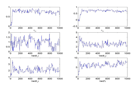
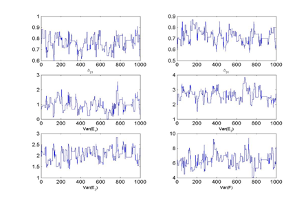
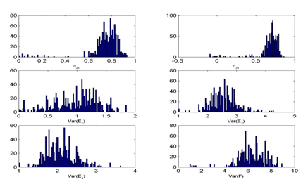
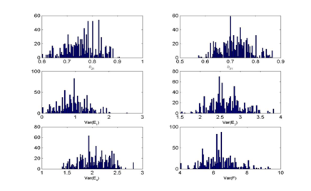
Figure 2 MCMC Chain histories and posterior densities for Model 1 (One Factor Model) parameters under arbitrary and ML starting values.

Clearly, with arbitrary staring values the burn-in phase is approximately 100 iterations while it is much shorter under the ML starting values. That is, using ML starting values one may not need any burn-in burn in period in this case and may be able to save the entire chain history. Note that the burn-in period of 100 iterations is rather short in this example due to the simple model chosen, but the difference between the starting values holds up for more complex models as well. This can be seen in the burn-in lengths in Table 2 for Model 2, for example. We will discuss the model complexity issue more in later part of this article.

Choice of jump size for proposal distribution

For illustration purposes, consider estimating Model 1 under all three jump size conditions. Figure 3 depicts the chain history and posterior distributions for 10,000 draws for all Model 1 parameters with the small and large jump size value options using the ML starting values.

Small Jump Size                Large Jump Size

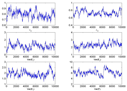
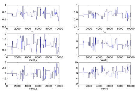
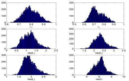
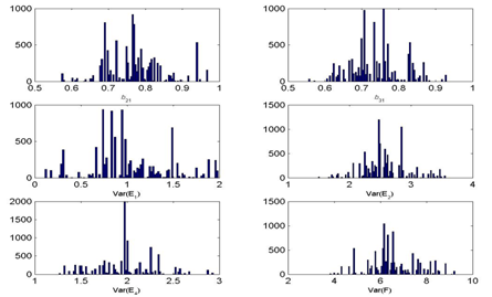
Figure 3 MCMC Chain histories and posterior densities for Model 1 (One Factor Model) parameters under small and large jump sizes.

As seen in Figure 3, under the small jump size option, all parameter chains fluctuated by only small amounts throughout the 10,000 iterations, which is also known as a slow mixing process. Specifically, an inspection of the actual samples taken, one can observe, for example, that all first 15 proposed values were accepted. Moreover, across entire 10,000 iterations for this scenario, the Metropolis acceptance rate is high at 88.40%. In the literature, an optimal range of 20-50% is recommended to achieve proper convergence^38,39 showing that the algorithm does not work as intended in this case.

Similarly, Figure 3 shows that the chains mix poorly under a large jump size as well. An inspection of the actual samples taken shows the opposite pattern for this jump size value than what was observed above. For example, all first 15 proposed values were rejected leading to an overall Metropolis acceptance rate of only 0.048% across all 10,000 iterations. Again, this rate is far from the optimal range of 20-50% recommended in the literature. In contrast, using a medium jump size for the proposal distribution leads to a proper mixing and an overall acceptance rate of 18.59% in this scenario; Table 4 shows the first 20 iterations for this model with 5 out of the 20 values accepted.

Despite the optimal performance of the medium jump size for the proposal distribution under ML starting values compared to other conditions, one may wonder whether this poor performance cannot be compensated for by simply increasing the number of iterations. Indeed, this is the case. To illustrate the point, Table 5 shows a summary of key posterior distribution characteristics such as their mean, variance, 2.5^th and 97.5^th percentiles under a variety of estimation conditions.

As Table 5 makes clear, when a small jump size and arbitrary starting values – both poor estimation choices – are coupled with 1,000,000 MCMC iterations, the resulting distributional characteristics are essentially indistinguishable from when a medium jump size and ML starting values are chosen – both more optimal choices – coupled with a cycle length of only 10,000 iterations.

In other words, if one is running very long MCMC runs, the impact of starting value and/or jump size onto the marginal density estimates will diminish as the MCMC run increase. However, the 1,000,000 MCMC iterations took 21 minutes to run on a Windows machine (Intel Core 2 Duo 2.00 GHz CPU with 777 MHz 1.99 GB of RAM), which is more than 100 times longer than the 10,000 MCMC run scenario, which took only 12.5 seconds.

Impact of model complexity

Consider further that Model 1 is an extremely simple SEM model – in fact, it is the simplest possible confirmatory factor model that could be estimated – suggesting that the effects observed here will be exacerbated for more complex SEM models. To illustrate this point, consider the case when Model 2 is run under the more optimal estimation conditions of medium jump size and ML starting values. First, even though the model is only slightly more complex than Model 1 conceptually, the overall Metropolis acceptance rate is only 6.52% across 10,000 iterations under these conditions as seen in Table 2. Note that this rate is out of the suggested optimal range 20-50% whereas that of model 1 was very close (19.97%) to the range. The increased model complexity considerably dropped convergence in terms of the Metropolis acceptance ratio. Second, as seen in Figure 4, the approximate burn-in size for this case is almost 3,000 which is 30 times more than that of the model 1. Third, Model 2 (e.g., 25.1 seconds) requires more than double CPU time than Model 1 (e.g., 12.3 seconds).

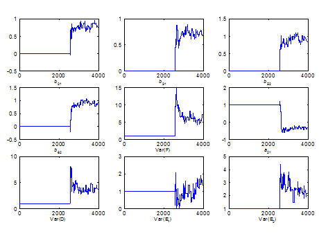
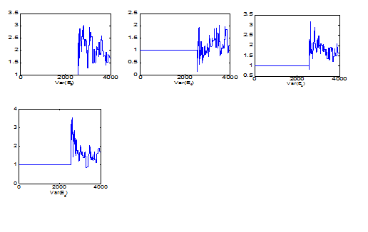
Figure 4 The first MCMC 4,000 iterations for Model 2 (Two Factor Model) parameters under medium jump sizes and arbitrary starting values.

Also note that this model complexity issue become more critical with bad (i.e., non-optional or un-tuned) starting values and/or jump sizes as seen in Table 2. For example, for both arbitrary starting value with medium jump sizes and ML starting values with large jump sizes cases, the Metropolis acceptance rates were 0%. In other words, the Metropolis sampler does not accept any proposed values during the entire MCMC run with 10,000 iterations. Thus, the burn-in period should be larger than 10,000 iterations. These results show how the model complexity can critically impact the MCMC estimation and underscore that it is imperative to develop “tuned” MCMC algorithms for SEM models, especially given the complexity of many SEM models in practice.

This article provided an accessible illustration of how different estimation choices impact how efficiently the Metropolis algorithm for MCMC estimation works in practice. Starting values for model parameters, jump sizes for the proposal distribution in the sampler, and complexity of the SEM model were varied in this paper to understand the consequence of these estimation conditions for the MCMC estimation results. The results in this paper showed how un-tuned starting values (i.e., an arbitrary starting value) and un-tuned jump sizes (i.e., jump sizes that are either too small or too large) for the proposal distribution that are result in slow and/or poor convergence.

The results show that “tuning” a sampling algorithm to achieve good mixing for a complex model is a challenging task, both computationally and mathematically (Gilks et al.,³⁰). Since the Metropolis algorithm has been introduced, more than dozens of MCMC algorithms have been developed during last three decades, which represent refinements of the algorithm for particular model structures. These algorithms include, among others, the Metropolis-Hastings algorithm (Hastings,⁴⁰), the Gibbs sampler (Gelfand & Smith;⁴¹ Geman, & Geman,⁴²), and the hybrid Monte Carlo algorithm (Duane, et al.,⁴³).

What this paper has shown is it is imperative to develop “tuned” MCMC algorithms so that they are well fitted for estimating SEM models, especially given the complexity of popular SEM models in practice. There currently is a practical disconnect between the technical advantages of MCMC over gradient-based estimation approaches, which have been well documented for decades, and meaningful advice for practitioners who want to understand how MCMC estimation works.

This paper was only illustrative, however. As such, it is limited in scope because (a) it discussed only the Metropolis algorithm, (b) used only the Wishart likelihood function, (c) used only a normal distribution function, (d) used only two simple SEM models, (e) used only selected estimation choices, and (f) focused only on selected outcome graphics and statistics. Nevertheless, as an illustrative paper, it makes two contributions to the emerging SEM literature on MCMC estimation. First, both numerical and conceptual details of MCMC estimation mechanisms with hands-on examples were provided to enhance the practical know-how of MCMC estimation for SEM specialists and to provide a more intuitive understanding of MCMC estimation process. Second, this article provided information regarding the consequence of various facets of MCMC estimation as a consciousness-raising device to illustrate that implementing MCMC estimation in latent variable modelling area is not as straightforward as some authors (e.g., Patz & Junker,^44-46) make it seem.

1. Bollen KA. Structural equation modeling with latent variables. Wiley, USA. 1989.
2. Browne MW. Generalized least-squares estimators in the analysis of covariance structures. South African Statistical Journal. 1974;8:1‒24.
3. Browne MW. Asymptotically distribution-free methods for the analysis of covariance structures. British Journal of Mathematical and Statistical Psychology. 1984;37(1):62‒83.
4. Gelman A, Carlin JB, Stern HS, et al. Bayesian data analysis. Chapman/Hall, USA, 1995.
5. Lee SY. Structural Equation Modeling: A Bayesian Approach. West Sussex: John Wiley & Sons Ltd. 2007.
6. Choi J, Levy R. Markov chain Monte Carlo Estimation Methods for Structural Equation Modeling: A Comparison of Subject-level Data and Moment-level Data Approaches. Biometrics and Biostatistics International Journal. 2017;6(5):00182.
7. Levy R, Mislevy RJ. Bayesian Psychometric Modeling. FL: Chapman & Hall/CRC, Boca Raton, USA, 2016. 
8. Junker B. Beyond MCMC. Paper presented at the annual meeting of the Psychometric Society (IMPS), USA, 2008.
9. Chen J, Choi J, Stapleton L, et al. An Empirical Evaluation of Mediation Effect Analysis with Manifest and Latent Variables using Markov chain Monte Carlo and Alternative Estimation Methods. Structural Equation Modeling: A Multidisciplinary Journal. 2014;21(2).
10. Kim JS,  Bolt DM. Estimating item response theory models using Markov chain Monte Carlo methods. Educational Measurement: Issues and Practice Volume. 2007;26(4):38‒51.
11. Lynch SM. Introduction to applied Bayesian statistics and estimation for social scientists. Springer, New York, USA, 2007.
12. Spiegelhalter DJ, Thomas A, Best NG, et al. BUGS: Bayesian inference Using Gibbs Sampling, Version 0.5, (version ii). Cambridge Medical Research Council Biostatics Unit. 1996.
13. Arbuckle JL. Amos 7.0 User's Guide. SPSS Inc, USA. 2006.
14. Metropolis N, S Ulam S. The Monte Carlo method. Journal of American Statistical Association. 1949;44(247):335‒341.
15. Metropolis N, Rosenbluth AW, Rosenbluth MN, et al. Equations of state calculations by fast computing machines. Journal of Chemical Physics. 1953;21(6):1087‒1091.
16. Jöreskog KG. A general approach to confirmatory maximum likelihood factor analysis. Psychometrika. 1969;34(2):183‒202.
17. Kennedy WJ, Gentle JE. Statistical computing. Marcel Dekker, New York, USA. 1980.
18. Süli E, Mayers D. An Introduction to Numerical Analysis. Cambridge University Press, India. 2003.
19. Choi J, Kim S, Chen J, et al. A Comparison of Maximum Likelihood and Bayesian Estimation for Polychoric Correlation using Monte Carlo Simulation. Journal of Educational and Behavioral Statistics. 2011;36(4):523‒549.
20. Choi J, Dunlop M, Chen J, et al. A Comparison of Different Approaches for Coefficient Alpha for Ordinal Data. Journal of Educational Evaluation. 2011;24(2):485‒506.
21. Andrieu C, Freitas N De, Doucet NA, et al. An introduction to mcmc for machine learning. Machine Learning. 2003;50:5‒43.
22. Dyer M, Frieze A, Kannan R. A random polynomial-time algorithm for approximating the volume of convex bodies. Journal Association Computing Machines. 1991;38(1):1‒17.
23. Jerrum M, Sinclair A. The Markov chain Monte Carlo method: an approach to approximate counting and integration. In: Hochbaum DS (Ed.), Approximation algorithms for NP-hard problems, PWS Publishing. Massachusetts. 1996;482‒519.
24. Arminger G, Muthén BO. A Bayesian approach to nonlinear latent variable models using the Gibbs sampler and the Metropolis-Hastings algorithm. Psychometrika. 1998;63(3):271‒300.
25. Lee SY, Song XY. Model comparison of nonlinear structural equation models with fixed covariates. Psychometrika. 2003a;68(1):27‒47.
26. Lee SY, Song XY. Bayesian model selection for mixtures of structural equation models with an unknown number of components. Br J Math Stat Psychol. 2003b;56(Pt 1):145‒165.
27. Scheines R, Hoijtink H, Boomsma A. Bayesian estimation and testing of structural equation models. Psychometrika. 1999;64(1):37‒52.
28. Shi JQ, Lee SY. Bayesian sampling-based approach for factor analysis models with continuous and polytomous data. British Journal of Mathematical and Statistical Psychology. 1998;51(2):233‒252.
29. Song XY, Lee SY. Bayesian estimation and test for factor analysis model with continuous and polytomous data in several populations. British Journal of Mathematical and Statistical Psychology. 2001;54(2):237‒263.
30. Song X, Lee SY. A Bayesian approach for multigroup nonlinear factor analysis. Structural Equation Modeling: A Multidisciplinary Journal. 2002;9(4):523‒553.
31. Gilks WR, Richardson S, Spiegelhalter DJ. Introducing Markov chain Monte Carlo. In: Gilks WR & Richardson S (Eds.), Markov chain Monte Carlo in practice, Chapman and Hall. 1996;1‒19.
32. Levy R, Choi J. An introduction to Bayesian Structural Equation Modeling. In: GR Hancock & RO Mueller (Eds,) Structural Equation Modeling: A Second Course (2nd edn), CT: Information Age Publishing, Inc, Greenwood, India. 2013.
33. Tierney L. Markov chains for exploring posterior distributions. The Annals of Statistics. 1994;22(4):1701‒1762.
34. MATLAB 6.5. MathWorks Inc, Natick, Massachussetts, USA. 2002.
35. Bentler PM, Wu EJC. EQS 6.1 for Windows. Encino, CA, USA. 2004.
36. Reisenzein R. A structural equation analysis of Weiner's attribution-affect model of helping behavior. Journal of Personality and Social Psychology. 1986;50:1123‒1133.
37. Weiner B. May I borrow your class notes? An attributional analysis of judgments of help giving in an achievement-related context. Journal of Educational Psychology. 1980;72(5):676‒681.
38. Roberts GO, Gelman A, Gilks WR. Weak Convergence and Optimal Scaling of Random Walk Metropolis Algorithms. Annals of Applied Probability. 1997;7(1):110‒120.
39. Roberts GO, Rosenthal JS. Optimal scaling of discrete approximations to Langevin diffusions. Journal of the Royal Statistical Society, Series B, Methodological. 1998;60(1):255‒268.
40. Hastings WK. Monte Carlo sampling methods using Markov chains and their applications. Biometrika. 1970;57(1):97‒109.   
41. Gelfand AE, Smith AFM. Sampling-based approaches to calculating marginal densities. Journal of the American Statistical Association. 1990;85:398‒409.
42. Geman S, Geman D. Stochastic relaxation, Gibbs distribution and Bayesian restoration of images. IEE Transactions on Pattern Analysis and MachineIntelligence. 1984;6(6):721‒741.
43. Duane S, Kennedy AD, Pendleton BJ, et al. Hybrid Monte Carlo. Physics Letters B. 1987;195(2):216‒222.
44. Patz RJ, Junker BW. Applications and extensions of MCMC in IRT: Multiple item types, missing data, and rated responses. Journal of Educational and Behavioral Statistics. 1999a;24(24):342‒366.
45. Patz RJ, Junker BW. A straight forward approach to Markov Chain Monte Carlo methods for item response models. Journal of Educational and Behavioral Statistics. 1999b;24(2):146‒178.
46. Lee SY, Song XY. Evaluation of the Bayesian and maximum likelihood approaches in analyzing structural equation models with small sample sizes. Multivariate Behavioral Research. 2004;39(4):653‒686.