Bifurcation analysis is a powerful tool as it allows one to identify in a systematic way where dynamics of interest exist in parameter space. Regions of stable solutions can be determined by computing stability boundaries directly as functions of the relevant system parameters. Sudden qualitative behavior changes in dynamical systems arise as a parameter is changed, which is known as bifurcation analysis.
Spruce budworms (Choristoneura fumiferana) are dangerous defoliators of forest lands in North America.1 These forests known as coniferous forests have pines, spruces, firs, and larches and the spruce budworm at larvae stage start feeding on needles of these trees. Fully grown insects can go through a tree in a time span of 4-5 years since they eat photosynthetic tissue which is crucial for the development of trees. The population usually stays at a low level in and less forestland because of their avian predators. But every three-four decades there is an outbreak of budworms and it results in a completely destroyed forest. It is assumed by scientists that this phenomenon has been occurring for more than thousands of years. Some papers that have studied bifurcation on various ecological models.1-4
The dynamics of one dimensional ordinary differential equations are not very diverse, like solutions either converge to a stable equilibrium or diverge. Geometric approaches give better insight on these models. As control parameter is varied bifurcations like saddle node bifurcations, transcritical bifurcation and pitchfork bifurcation occur. When two fixed points annihilate each other or reappear as a parameter is changed it is known as saddle node bifurcation. Transcirital bifurcation is when a steady equilibrium changes its stability. And pitchfork bifurcation works with symmetry, fixed points disappear or appear in symmetric pairs.
The dispersal dynamics of prey-predator, competition, and mutualism is explored in.5 A very recent study of diffusion reaction in competition model is.6 There are also other studies7-9 related to diffusion where the effect of dispersion procedures on competitive populations are explored. In another study, the relation between growth rates, carrying capacity, and diffusion strategies is discussed, it is analyzed in9 whether coexistence is promoted when diffusion strategies are diverse. Here bifurcation analysis will be used to understand why this happens thus giving a mathematical point of view on this phenomenon.
In this paper, we have an elementary discussion on bifurcations in one-dimensional ordinary differential equations. Graphical methods are used to identify equilibrium points, determine their stability, and to see the behaviors of the numerical solutions near fixed points.10-12 In section 2, the general forms of bifurcations in autonomous differential equations such as Saddle node bifurcation, transcritical bifurcation, and pitchfork bifurcation will be analyzed. Following this discussion, in section 3 the mathematical model for spruce budworm for single species pray is explored. We talk thoroughly about the function for the rate of predation. In section 4 a dimensionless model is going to be introduced for further analysis of the model. Further into the paper, in section 5 we look into bifurcations that occur in the spruce budworm model when change of parameter values occur. In section 6 we studied harvesting in population models, we took different levels of harvesting into consideration, leading us to the conclusion.
Bifurcation Preliminaries
In this section we have discussed about some common bifurcation behavior.
Pitchfork Bifurcation
Consider the following equation for the classic form of the Pitchfork Bifurcation in one dimensional
form:
(1.1)
Pitchfork bifurcation is a local type of bifurcation that deals with symmetry, where equilibrium points show up or dissipate in pairs.14,15 In Figure 1 we see the vector field of equation (1.1) for multiple values of α. First, when
and
there is only one fixed point, and it stable for both times. But when the value of α is increased to two new equilibrium points appear, and the stability at
changes. The new two fixed points are stable, and this will be true for all
as the fixed points will be symmetrically positioned at
.

Figure 1 Pitchfork bifurcation.
The stable lines in Figure 2 are given by
when
and
. The origin becomes unstable for α>0 and that is shown using the dotted line. Some other bifurcations are discussed and can be found in Appendix.
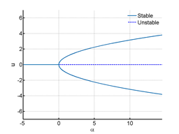
Figure 2 Bifurcation diagram for Pitchfork bifurcation.
Spruce Budworm mathematical model
In this study, we propose the following spruce budworm model3,10 for a single species prey:
(2.1)
where r is the intrinsic growth rate of the spruce budworm.
is the carrying capacity, which
depends on the availability of the foliage of the balsam firs. The rate of predation
(2.2)
is from avian predators, which associate reward with prey, a learned behavior. They focus on their best sources of prey, which allows a low density prey to escape notice. The functional form of this type of predation follows the Holling’s Type III S-shaped response as defined by
.3,10,14 represents the saturation level of the predator, e.g., constant population can eat so much prey, this saturation level works like an upper limit on the predation. α determines the densities of spruce budworm that cause avian predation. Now if taking the limiting value of the predation function,
From Figure 3 it is seen that the function is monotonically increasing until it reaches its asymptote at the value β.3 This indicates that no matter how much the budworm population increases the birds can eat a limited quantity. Using basic calculus, the first and second derivative is calculated to find the point of inflection. This point determines when the budworm population increases rapidly.
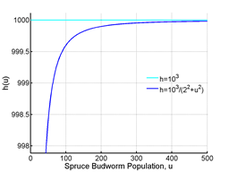
Figure 3 Rate of Predation.
Differentiating equation (2.2) with respect to u,
(2.3)
It is obvious that h^' (u)>0 since all the constants are positive. Now again differentiating with
respect to ,
(2.4)
Substituting equation (2.4) to zero, yields,
(2.5)
Population cannot be negative so the negative is omitted. Thus predation dramatically climbs upwards to
from below. After crossing the point of inflection, the function gradually approaches its asymptote at
.
Dimensionless Model
In order to simplify the differential equation and analyze the behavior better we reduce the number of parameters. Let,
Substituting the above values in (2.1),
(2.6)
If
, from equation we have,
(2.7)
Assume that
, then from equation (2.7) we get,
Defining the new scaled parameters
and
. Then the dimensionless model is given by,
(2.8)
To find the equilibrium points, let
, then,
(2.9)
Consider the function,
and
. Thus
is a trivial equilibrium point. In order to find the other equilibrium points we will graph
and
and look at the intersection points. Here,
=Per capita growth rate of the scaled population variable
with respect to scaled time
=α.
=Per capita death rate of the spruce budworm due to avian predation.
Bifurcation Analysis
Qualitative changes in dynamical systems, like fixed points being created and destroyed or their stability changing is called bifurcation. In one dimensional systems these alterations occur when a parameter value is changed. Here we will see a practical example of saddle node bifurcation. We will plot
and
for different values of the parameters involved in the equation and look for fixed points. The stability of a fixed point is determined by reading the direction of the flow on
axis. If
then the flow is to the right otherwise it is directed to the left. Now if the flow is inwards then the point is stable and if the flow is outwards then the point is unstable.10 We will also plot the numerical solutions of the autonomous equation. First we start with small values of
and
. From the Figure 4 it is seen that there is only one fixed point at
and it is stable. On the right figure the numerical solutions for equation from various initial values and all of the solution gradually converge towards equilibrium solution. At this stage the budworm population stays limited.
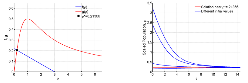
Figure 4 For R=0.22 and C=3.
Here in Figure 5 the value of is increased 0.8 to and
. Despite this huge increment it is seen from the Figure 5 that the number of fixed points remain the same. This fixed point is also stable, the value is very low and the budworm population remains endemic.
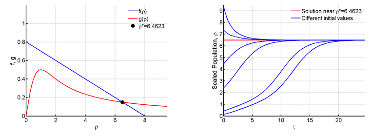
Figure 5 For R=0.8 and C=8.
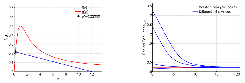
Figure 6 For R=0:22 and C=12.
We will increase C to a higher value of and change R values. Since the parameter C is acquainted with the carrying capacity K, holding C at a higher value will help us analyze the model when the forest is large. Starting at
we see that the results are quite similar to the ones obtained at Figure 4.
Next in Figure 7 we can see that when we raise R to 0.32 there is one fixed point at
and the function is
tangent to
at 5.82579. A saddle-node bifurcation is thus occurring.
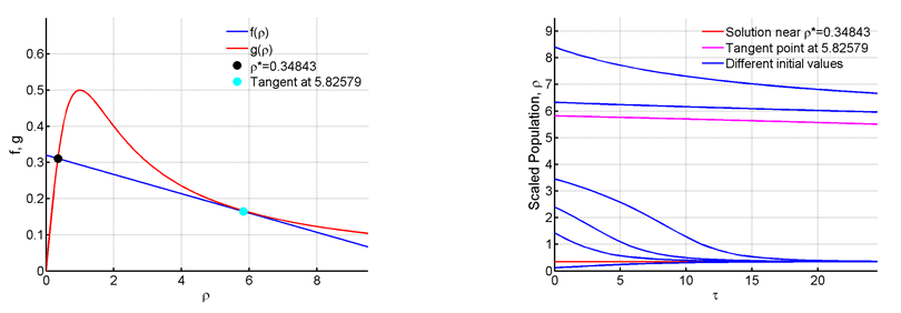
Figure 7 For R=0.32 and C=12.
As R continues to escalate to 0.45 we see from Figure 8 that two new fixed points have emerged at 2.32714 and 9.10661. Here the point 2.32714 is unstable since at the left of the point
and the flow is outwards. On the right
and the flow is inwards.10 The following fixed point is of course stable. Since two stable points or unstable points cannot occur side by side. As for the numerical solutions the solution curves remain close to the stable equilibria. Values that are larger than the unstable fixed point approaches the larger stable fixed point at
and values less than it approach the stable point occurring at a low value.

Figure 8 For R=0.45 and C=12.
In figure 9 we notice that a new saddle-node bifurcation arises. The two points 0.56624 and 2.32714 gradually approach each other and collide into a new fixed point at 9.78531, as R is raised to 0.548. The fixed point at 0.49743 is stable, but at a very high value.15 Which causes an outbreak in the spruce budworm population.

Figure 9 For R=0.548 and C=12.

Figure 10 For R=0.6 and C=12.
Now at
and the saddle node bifurcation disappears and there is only one stable fixed point at 10.02456.
Population models with harvesting
In this section we will analyze the behavior of the logistic population model when population is removed at some defined rate, more commonly known as harvesting.16 The harvesting function is defined as , dependent on time
.
Calibration of the model with constant harvesting
Let us consider the following model,
(3.1)
Equation (3.1) is a population model with constant-yield harvesting. We would like to study this model and see how different harvesting levels affect the model. Some real-life examples are harvesting animals like deers, birds from sanctuaries, or even fishes, for example whales. In these sort of scenarios harvesting is allowed to some limited extent.
In Figure 11, we have plotted
for different values of H. Now solving eqaution (3.1) analytically yields a very complicated structure, so we approach a graphical method to obtain the steady states. Solving the quadratic equation,
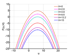
Figure 11 F(u,H) for different values of H.
(3.2)
We get
. Now when
that is,
the quadratic equation (3.2) has two real roots, giving two fixed points for the model. H=0 and H=2.6 represents this case. When H=0 the model is constituted as the logistic growth model. Now when H=2.6 there are two fixed points, the one at
is unstable and the latter fixed point at
is stable (Figure 12). For initial values, when
the solutions move away from the unstable equilibrium, known as the extinction equilibrium and approach the solution curve near
. But for initial values less than
the solutions approach negative infinity, thus the population declines.

Figure 12 Numerical solutions for different values of H.
Next when H=4.8 a saddle node bifurcation occurs, two fixed points collide into one at
. This fixed point is half stable. The numerical solutions are observed in the second plot Figure 12 shows us that for initial values less than the solutions diverge, but when they are greater than they move towards the equilibrium. Gradually as H is increased, that is when
all the fixed points disappear and the solutions diverge. Thus for harvesting,
the population fails to survive.
Calibration of the model with proportional harvesting
Here, we now consider the following equation,
(3.3)
In Figure 13 we have plotted
for various values of .
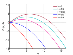
Figure 13 G(u; H) for different values of H.
Solving equation (3.3) for equilibrium points we get,
From equation (6.4) we have u = 0 is always an equilibrium point and the other one is
. When
we have two fixed points. The extinction equilibrium at
and
. From the first plot in Figure 14 we observe that
is the stable
equilibrium. This case is true for all
, that is when
here
.
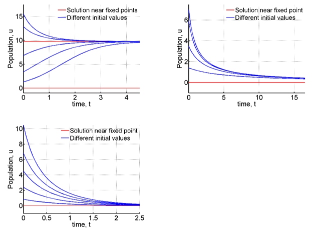
Figure 14 Numerical solutions for different values of H.
When H is increased to 1.6 transcritical bifurcation occurs and
is the only fixed point which is half stable. For
or in this case
, the extinction equilibrium becomes stable and the other fixed point is negative. Thus when
, harvesting is too intense and it surpasses population growth.


