Parametric and non-parametric bootstrap methods are used to investigate the statistical properties of the dissolution similarity factor $f_2$. The main objective of this study is to compare the results obtained by these two methods. We estimate characteristics of the sampling distribution of ${\widehat{f}}_2$ statistic under these methods with various bootstrap sample sizes using Monte Carlo simulation. A number of bootstrap confidence interval (CI) construction techniques are used to determine a 90 % CI for the true value of $f_2$under both parametric and non-parametric schemes. The bootstrap sampling distributions of ${\widehat{f}}_2$ under both schemes are found to be approximately symmetrical with a non-zero excess of kurtosis. Non-parametric bootstrap confidence intervals for $f_2$ perform better than those obtained from parametric methods. The Bias corrected (BC) and accelerated bootstrap percentile (BCa) confidence interval method produce more precise two-sided confidence intervals for $f_2$compared to other methods

Keywords: dissolution profiles, bootstrapping, confidence interval, bias-corrected and accelerated bootstrap percentile confidence interval

In pharmaceutical studies for solid and oral drugs, it is important to compare a test drug to a reference drug using average dissolution rates over time. The purpose of dissolution testing is to develop a new formulation, to ensure quality control, and to assess stability and reproducibility of the immediately released solid oral drug.^1‒3 Assessment of dissolution profiles for two drugs, in vitro, provides the waiver for in-vivo assessment.

The United States Food and Drug Administration (FDA) requires similarity tests for the dissolution profiles of two drugs under consideration when there are post drug-approval changes. Such changes include change of manufacturing sites, change in formulations, and change in component and composition. Despite the post-approval changes, two drugs are similar with respect to their dissolution rates if the test (post-approval) has the same (equivalent) dissolution performance as the reference (pre-change).

In order to assess drug dissolution profiles, both model-dependent and model-independent methods are used. In a model-dependent approach, an appropriate mathematical model is selected to describe the dissolution profiles of the two drugs. The model is then fit to the data and confidence intervals for the model parameters are constructed. These confidence intervals are then compared with the specified similarity region. Commonly used model-dependent methods to fit the dissolution profiles include Gompertz,⁴ Logistic,⁵ Weibull,⁶ probit and sigmoid models.^7,8 Model-dependent methods have some limitations. For example, selecting an appropriate model, and interpreting its parameters are difficult when the dissolution profiles for the two drugs follow different models.

To overcome the limitations of model-dependent approaches, model-independent approaches such as difference factor$f_1$, similarity factor$f_2$, analysis of variance, split plot analysis, repeated measure analysis, Hotelling $T^2$, principal component analysis1 and first order autoregressive time series analysis are used. Among these methods, analysis of variance, split plot analysis assume that dissolution data are independent over time. These two methods are not appropriate in many cases as data are not independent. As an alternative, Tsong et al.,⁹ proposed Hotelling $T^2$ statistic to construct a 90% confidence region for the difference in dissolution means of two batches of the reference product at two time points. This confidence region is then compared with a pre-specified similarity region.

Of all the model-independent approaches, the US FDA recommends only $f_2$¹⁰ to study similarity between two drug dissolution profiles under consideration. Although this similarity factor $f_2$ is used to assess global similarity of dissolution profiles, and it does not require any assumption regarding data generating process, using point estimate of $f_2$in comparing two drug dissolution profiles is not appropriate if there is substantial variation from batch to batch. In this case, it is necessary to construct the confidence intervals for$f_2$. Construction of confidence interval for $f_2$ depends on the standard error of its estimator${\widehat{f}}_2$. Since there is no closed form formula for the standard error of${\widehat{f}}_2$, and hard to derive analytically, we approximate the standard error of ${\widehat{f}}_2$ by deriving sampling distribution of ${\widehat{f}}_2$ using parametric and non-parametric bootstrap methods. Then the approximated standard error of ${\widehat{f}}_2$ is used to construct bootstrap confidence intervals for$f_2$.

The organization of this paper is as follows: in section 2 we present basic characteristics of drug dissolution data used in our study and chi-square plot for assessing the normality of the underlying population of the data. Section 3 discusses the statistical framework used in dissolution testing and gives an outline how two drugs are considered to be similar in terms of dissolved drug ingredients into the media. In section 4, bootstrap methods are briefly discussed and related confidence intervals for the true value of ${\widehat{f}}_2$ are presented. Section 5 discusses the results of our study and section 6 concludes the paper.

We consider the standard dissolution data discussed by Chow & Liu,¹¹ Tsong^12,13 to assess the various characteristics of ${\widehat{f}}_2$. The Summary measures of the reference and the test drug dissolution data are presented in Table 1.

The observed difference between mean dissolution rate factors, $f_2$for the test and the reference drug at different time points are less than 10 percent. The standard deviation of the dissolution rate factor at different time points for the test and the reference drug are also less than 10 percent. The mean differences between the two drugs are wider at the starting time points than in the mid-time points. Figure 1 shows dissolution profiles for the test and the reference drugs.

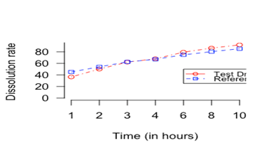
Figure 1 Dissolution profiles for the test and the reference drugs

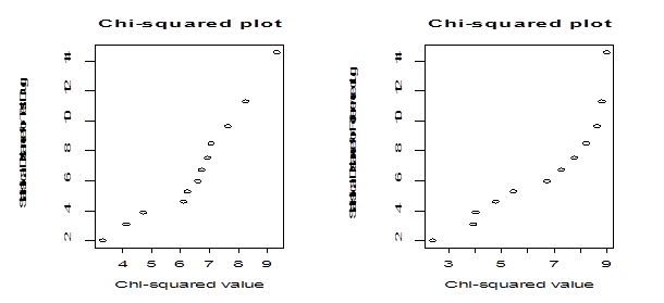
In order to perform parametric bootstrapping using the above data, we need to know the parametric form for the distribution of the population from which these sample dissolution factors are drawn. In particular we check if the sample dissolution factors are drawn from multivariate normal distribution. To check normality, we examine the underlying distribution of the data using a chi-square plot and a normality goodness of fit test. Because the observations from the same tablets across time are related and the observations across the tablets at a fixed time point are independent, the dissolution data used in this article are considered to be a realization of multivariate observations. To check whether the dissolution data we consider for our study come from the multivariate normal distribution, we calculate statistical distance measures and use them to construct a chi-square plot under the normality assumption (Figure 2).

Figure 2 Left panel: Chi-square plot for the test drug. Right panel: chi-square plot for the reference drug

Since the points in plots are not on a straight line, we say that the data do not follow multivariate normal distributions. We also use the formal correlation test to measure the straightness of the Q-Q plot. The values of the correlation coefficient for the Q-Q plot for the test and the reference drug dissolution data are 0.95 and 0.91 respectively. At 5% level of significance the tabulated value of the correlation coefficient for sample size of $n=12$ is 0.9298. For the test drug dissolution data, the normality assumption is reasonable but for the reference drug, normality assumption is off slightly.

Let $y_{ijt}$ be the percentage of drug dissolved in a media at time point t from the tablet i for drug j. Then the statistical model for the drug dissolution percentage can be written as$y_{ijk}={\mu }_{jt}+{\epsilon }_{ijt}$, $t=1,2,\mathrm{...},T$; $i=1,2,\mathrm{...},n$; $j=1,2.$ Here ${\mu }_{jt}$is the population mean over tablets at time t for drug $j$ and ${\epsilon }_{ijt}$ has mean 0. Since the dissolution percentage is measured over time from the same tablet of the drug, the measurements are dependent. However, it is reasonable to assume that the $n$ vectors $y_{1j},y_{2j},\mathrm{...},y_{nj},j=1,2$ are independent, as these are replications across tablets in the population. The dissolution profiles (Figure 1) of the test drug and the reference drug are considered to be similar if and only if the population means vector for the test drug is in some neighborhood of the population mean vector for the reference drug. A rectangular similarity measure recommended and required by FDA is used to assess if two drugs are similar. This similarity measure is$\left|{\mu }_{1t}-{\mu }_{2t}\right|\le \Delta$, where $\Delta$ a specified number is. Generally FDA recommends that the specified number is 10 for all time point. A similarity measure $f_2$, based on the rectangular measure and recommended by FDA, is discussed in Section 3.1.

Similarity factor $f_2$

Moore et al.,¹⁰ developed a similarity factor, $f_2$, for testing dissolution profiles of a test and a reference drug.

The$f_2$ similarity factor is defined as

$f_2=50\log \left\{100{\left(1+D^2\right)}^{-\frac{1}{2}}\right\}$,

where$D^2=\frac{1}{T}{\displaystyle \sum _{t=1}^T{\left({\mu }_{1t}-{\mu }_{2t}\right)}^2}$and${\mu }_{jt}$is population mean dissolution rates over time $t\left(t=1,2,\mathrm{...},T\right)$and for the $j\text{th}$drug$\left(j=1,2\right)$. $D^2$is a squared distance from the population mean vector of the test drug to the population mean vector of the reference drug. Since dissolution measurements are expressed as percent, $D^2$ranges from 0 to${100}^2$.

The similarity factor $f_2$ is a monotone decreasing function of$D^2$ with a maximum of 100 when $D^2=0$ (two dissolution profiles are the same), and a minimum of 0, when$D^2={100}^2$.

A value of $f_2$ in the range of 50 to 100 ensures the similarity or equivalence of two dissolution profiles. When the rectangular similarity measure (adopted by FDA) is $\left|{\mu }_{2t}-{\mu }_{1t}\right|\le 10$ for all time points, then$f_2$ is very close to 50. So the similarity region in the range of 50 to 100 indicates the similarity of two drugs.

This similarity factor works well when the following conditions are met: (i) there is a minimum of three time points, (ii) there are 12 individual values for each time point for each formulation, (iii) no more than one mean value is greater than 85% dissolved for each formulation, and (iv) the standard deviation of the mean of any product is less than 10% from the second to last time points.

Bootstrap methods

Bootstrapping^14,15 is a computer-intensive approach to statistical inference. It is based on the sampling distribution of a statistic obtained by resampling from the data with replacement. When it is hard to derive the exact sampling distribution of certain statistics and their characteristics, bootstrap methods are used to approximate them. The characteristics include standard error, bias, skewness, critical values, mean squared error, and others. To derive an exact sampling distribution of a statistic of interest, the underlying population distribution from which sample is drawn has to be known. Sometimes even though the underlying distribution is known, derivation of the exact sampling distribution for certain statistic is not possible or is very complex. In such case, bootstrap methods allow estimating or approximating the sampling distributions of these statistics. The bootstrap approach does not require knowledge of the data generating process but uses the sample information only. The idea behind bootstrapping is that the use of sample information as a “proxy population”. One takes samples with replacement from the original sample and calculates the statistic of interest repeatedly. This leads to a bootstrap sampling distribution. This sampling distribution is used to measure the estimator’s accuracy and helps to set approximate confidence intervals for certain population parameters.

We use two types of bootstrap methods, parametric and non-parametric to determine the sampling distribution of the statistic ${\widehat{f}}_2$and its characteristics. Using both techniques we construct 90% confidence intervals for$f_2$. We briefly describe both methods as follows.

Let $X_1,X_2,\mathrm{...},X_n$be independent and identically distributed random variables from an unknown distribution ${\widehat{F}}_n$. $F$ is estimated using the empirical distribution ${\widehat{F}}_n$. Repeated samples are taken from the estimated empirical distribution${\widehat{F}}_n$. Then the statistic of interest is calculated using each bootstrap samples, giving a set of bootstrap values for the desired statistic. Using the bootstrap values of the statistic, the estimated distribution function and its properties are calculated. This approach is called non-parametric bootstrapping.

The parametric bootstrap, on the other hand, assumes that $F$is known except for its parameters.$F$is approximated by estimating the parameters with the sample observations. Then from the approximated distribution${\widehat{F}}_n$, repeated samples are taken. The values of the statistic of interest are calculated using these bootstrap samples. These bootstrap values of the statistic are used to derive the desired measures. Under both schemes, the distribution of ${\widehat{f}}_2$ can be estimated by using the bootstrap with the Monte Carlo approximation as follows.

$F(x)=\frac{1}{B}{\displaystyle \sum _{b=1}^{B}I\left\{f_2^{*}\le x\right\},}$

where $f_2^{*}$is the value of the $f_2$ based on the bootstrap sample and $F(x)$is a bootstrap estimator of the distribution function of ${\widehat{f}}_2$based on the data$X_1,X_{2,}\mathrm{...},X_n$. The bootstrap histogram for $\left\{f_2^{*},b=1,2,\mathrm{...},B\right\}$can be used to estimate the density of${\widehat{f}}_2$. The expected value, variance, skewness, kurtosis, and bias of the bootstrap sampling distribution of ${\widehat{f}}_2$ are estimated from$F(x)$. In order compute them, we first take B independent samples$\left\{X_1^{*,b},X_2^{*,b},X_3^{*,b},\mathrm{...},X_n^{*,b}\right\}$, $b=1,2,\mathrm{...},B$ and approximate them by

${\overline{\widehat{f}}}_2=\frac{1}{B}{\displaystyle \sum _{b=1}^B{f}_{2,b}^{*}}$, ${\upsilon }_{\text{boot}}^{\left(B\right)}=\frac{1}{B}{{\displaystyle \sum _{b=1}^B\left(f_{2,b}^{*}-{\overline{\widehat{f}}}_2\right)}}^2$,

$s{k}_{\text{boot}}^{\left(B\right)}=\frac{\frac{1}{B}{{\displaystyle \sum _{b=1}^B\left(f_{2,b}^{*}-{\overline{\widehat{f}}}_2\right)}}^3}{{\left[{\upsilon }_{\text{boot}}^{\left(B\right)}\right]}^{\frac{3}{2}}}$, $k_{\text{boot}}^{\left(B\right)}=\frac{\frac{1}{B}{{\displaystyle \sum _{b=1}^B\left(f_{2,b}^{*}-{\overline{\widehat{f}}}_2\right)}}^4}{{\left[{\upsilon }_{\text{boot}}^{\left(B\right)}\right]}^2}$

and $b_{Boot}^{\left(B\right)}={\overline{\widehat{f}}}_2-{\widehat{f}}_2;$

here ${\overline{\widehat{f}}}_2$, ${\upsilon }_{\text{boot}}^{\left(B\right)}$, $s{k}_{\text{boot}}^{\left(B\right)}$,$k_{\text{boot}}^{\left(B\right)}$, and $b_{Boot}^{\left(B\right)}$ are Monte Carlo bootstrap estimator for mean, variance, skewness, kurtosis and bias of the sampling distribution of $\widehat{f}$ respectively. In section 4, we construct bootstrap confidence intervals for $f_2$ using a number of available bootstrap confidence interval methods.

An observed value of ${\widehat{f}}_2$ is used to assess whether two drugs (test and reference) are similar or not with respect to their dissolution profiles. This value is compared with the specifications given by the FDA in order to decide if the two drugs are similar. However, due to sampling variation, it is not reasonable to assess the dissolution similarity of two drugs by directly comparing ${\widehat{f}}_2$with the specification limits. Rather one can make a decision of dissolution similarity by constructing a 90% confidence interval for the population parameter$f_2=E({\widehat{f}}_2)$. In this section we use parametric and non-parametric bootstrap methods discussed in subsection 3.2 to construct the confidence intervals for$f_2$.

A detailed discussion on different types of bootstrap confidence intervals can be found in Chernick,¹⁶ Davison,¹⁷ DiCiccio,¹⁸ Efron.¹⁹ Here we review different types of bootstrap procedures used to construct confidence intervals for the parameter of interest briefly. For notational convenience, we denote the similarity parameter $f_2$as $\theta$ and $\widehat{\theta }$ as its estimate.

The standard bootstrap confidence interval is given by

$\left[\widehat{\theta }-z^{\left(\frac{\alpha }{2}\right)}s{\widehat{e}}_{({\widehat{\theta }}^{*})},\widehat{\theta }+z^{\left(1-\frac{\alpha }{2}\right)}s{\widehat{e}}_{({\widehat{\theta }}^{*})}\right]$

where $s{\widehat{e}}_{({\widehat{\theta }}^{*})}$ is the bootstrap standard error of the estimator $\widehat{\theta }$, and $z^{\left(\frac{\alpha }{2}\right)}$ is the $100.\frac{\alpha }{2}th$ quantile of the standard normal distribution. In percentile interval method of bootstrapping, $B$bootstrap estimates ${\widehat{\theta }}_b^{*}$$\left(b=1,2,\mathrm{...},B\right)$are generated. Then these bootstrap estimates are arranged in ascending order. If we denote $F\left({\widehat{\theta }}^{*}\right)$ as the cumulative distribution function of ${\widehat{\theta }}^{*}$, then a 90% percentile interval is defined by

$\left({\widehat{\theta }}_b^{*\left(\frac{\alpha }{2}\right)},{\widehat{\theta }}_b^{*\left(1-\frac{\alpha }{2}\right)}\right)=\left[{\widehat{F}}^{-1}\left(\frac{\alpha }{2}\right),{\widehat{F}}^{-1}\left(1-\frac{\alpha }{2}\right)\right]$

where $\alpha =5\%$ and ${\widehat{\theta }}^{*\left(\frac{\alpha }{2}\right)}$ indicates the $100.\frac{\alpha }{2}th$ percentile of $B$ bootstrap replications.

Although the computation is straightforward, this method does not work well when the sampling distribution of $\widehat{\theta }$ is skewed or $\widehat{\theta }$ is biased.^20,21

In the presence of skewness and bias, the percentile method can be improved by an adjustment to the percentile method. This bias adjusted and corrected percentile interval is known as bias corrected percentile interval method (BC).²² In the bias-corrected method, the observed amount of difference between the median of the bootstrap estimate ${\widehat{\theta }}^{*}$and the observed estimate from the original sample is defined as bias. The bias-correction constant estimate, denoted by${\widehat{z}}_0$, is defined as

${\widehat{z}}_0={\Phi }^{-1}\left(\frac{\#{\widehat{\theta }}^{*}<\widehat{\theta }}{B}\right)$,

where ${\Phi }^{-1}$ is the inverse function of a standard normal cumulative distribution function. Then, a $100\left(1-\alpha \right)$percent bias-corrected percentile confidence interval for $\theta$ is given by $\left[{\widehat{\theta }}^{*\left({\alpha }_1\right)},{\widehat{\theta }}^{*\left({\alpha }_2\right)}\right]$,

where

${\alpha }_1=\Phi \left(2z_0+z^{\left(\frac{\alpha }{2}\right)}\right)$
${\alpha }_2=\Phi \left(2z_0+z^{\left(1-\frac{\alpha }{2}\right)}\right)$.

Here $\Phi$ is the standard normal cumulative distribution function and $z^{\left(\frac{\alpha }{2}\right)}$ is the $100\frac{\alpha }{2}\text{th}$ percentile point of the standard normal distribution. Although the bootstrap bias correction improves the bootstrap percentile method with taking the bias into account, this method does not work well in some cases.²¹

Efron²² introduced a further improved bootstrap method that corrects the bias due to the non-normality and also accelerates convergence to a solution. The method corrects the rate of change of the normalized standard error of $\widehat{\theta }$ relative to the true parameter$\theta$. It takes into account the skewness in the distribution along with the bias of the estimator. This method is called bias-corrected and accelerated (BCa) percentile method. Chernick et al.,¹⁶ show that for small sample sizes BCa may not work as percentile method because the bias and acceleration constant must be estimated and the sample size is not large enough for asymptotic advantage of BCa to hold.

The BCa confidence interval for $\theta$ is

$\left[{\widehat{\theta }}^{*\left({\alpha }_1^{*}\right)},{\widehat{\theta }}^{*\left({\alpha }_2^{*}\right)}\right]$,

where

${\alpha }_1^{*}=\Phi \left({\widehat{z}}_0+\frac{{\widehat{z}}_0+z^{\left(\frac{\alpha }{2}\right)}}{1-a\left({\widehat{z}}_0+z^{\left(\frac{\alpha }{2}\right)}\right)}\right)$ and

${\alpha }_2^{*}=\Phi \left({\widehat{z}}_0+\frac{{\widehat{z}}_0+z^{\left(1-\frac{\alpha }{2}\right)}}{1-a\left({\widehat{z}}_0+z^{\left(1-\frac{\alpha }{2}\right)}\right)}\right)$,

where $\Phi$ is the standard normal cumulative distribution function and $z^{(.)}$ is the percentile of standard normal distribution.

The bias correction term ${\widehat{z}}_0$ is calculated by $z_0={\Phi }^{-1}\left(\frac{\#\left({\widehat{\theta }}^{*}<\widehat{\theta }\right)}{B}\right)$, and the acceleration constant $a$is :

$a=\frac{{{\displaystyle \sum _{i=1}^n\left({\widehat{\theta }}_{(.)}-{\widehat{\theta }}_{\left(i\right)}\right)}}^3}{6{\left[{{\displaystyle \sum _{i=1}^n\left({\widehat{\theta }}_{(.)}-{\widehat{\theta }}_{\left(i\right)}\right)}}^2\right]}^{\frac{3}{2}}}$,

where ${\widehat{\theta }}_{(.)}$ and ${\widehat{\theta }}_{\left(i\right)}$are the average and $i\text{th}$jackknife estimate of the parameter.

The problem arising from the skewness in the sampling distribution of $\widehat{\theta }$ can also be handled by an alternative method called Bootstrap-t method.^22,26,27 The bootstrap-t method is defined by the pivotal quantity $t^{*}=\frac{{\widehat{\theta }}^{*}-\widehat{\theta }}{s{e}_{{\widehat{\theta }}^{*}}}$, where ${\widehat{\theta }}^{*}$ and $s{e}_{{\widehat{\theta }}^{*}}$ are the bootstrap estimator and its standard error. Since the standard error of $\widehat{\theta }$ is not known, it is estimated by Monte Carlo simulation. However, this simulation requires nested bootstrapping. For each bootstrap sample, we calculate $t^{*}$and these resulting $t^{*}$’s are placed in ascending order and select $100\left(\frac{\alpha }{2}\right)\text{th }$ and $100\left(1-\frac{\alpha }{2}\right)\text{th }$percentile values of $t^{*}$. Then, $100\left(1-\alpha \right)$percent bootstrap-t confidence for $\widehat{\theta }$ is

$\left[\widehat{\theta }-t_{1-\frac{\alpha }{2}}^{*}s{e}_{{\widehat{\theta }}^{*}},\widehat{\theta }-t_{\frac{\alpha }{2}}^{*}s{e}_{{\widehat{\theta }}^{*}}\right]$

where $\widehat{\theta }$ is estimate of the parameter $\theta$ from the original sample and $s{e}_{{\widehat{\theta }}^{*}}$is the bootstrap standard error.

Properties of the distribution of ${\widehat{f}}_2$

In this section, we examine the properties of the bootstrap sampling distribution of ${\widehat{f}}_2$ by using both non-parametric and parametric bootstrap sampling. To generate the bootstrap samples with non-parametric and parametric bootstrap methods discussed in subsection 3.3. the following algorithms are employed: (a) For Non-parametric bootstrapping: $B(b=1,2,\mathrm{...},B)$independent sample with replacement from the observed $y_{1j},y_{2j},\mathrm{...},y_{nj},j=1,2$are drawn and for each bootstrap sample $\widehat{f}$, which is the estimate of $f_2$defined in Subsection 3.1, is calucated; (b) For Parametric bootstrappping: $B$ independent samples are drawn from $N_T({\widehat{\mu }}_j,{\widehat{\sum }}_j),j=1,2$, where $\widehat{\mu }={({\widehat{\mu }}_{j1},{\widehat{\mu }}_{j2},\mathrm{...},{\widehat{\mu }}_{jT})}^T$ and ${\widehat{\sum }}_j$ of $T\times T$ covariance matrix are moment estimates of ${\mu }_j$ and ${\sum }_j$ and for each bootstrap sample ${\widehat{f}}_2$, the estimate of $f_2$ is calculated.

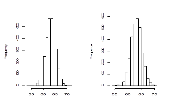
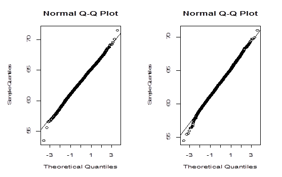
The histograms and Q-Q plots are constructed using the bootstrap values of ${\widehat{f}}_2$generated by both methods and are shown in Figure 3 & Figure 4 respectively.

Figure 3 Left panel: Histogram of 3000 parametric bootstrap of ${\widehat{f}}_2$. Right panel: Histogram of 3000 non-parametric bootstrap of ${\widehat{f}}_2$.

Figure 4 Left panel: Q-Q plot for the values of ${\widehat{f}}_2$ generated by parametric bootstrap method. Right panel: Q-Q plot for the values of ${\widehat{f}}_2$ generated by non-parametric bootstrap method.

The Bootstrap parametric and non-parametric sampling distributions of ${\widehat{f}}_2$shown in the left and right panels of Figure 2 are almost symmetrical. However, the non-parametric sampling distribution of the similarity factor${\widehat{f}}_2$is more symmetrical than that of the parametric one. In addition, the bootstrap parametric sampling distribution of ${\widehat{f}}_2$ is wider than the non-parametric bootstrapping. The percentile confidence methods work well if the underlying probability distribution from which samples are drawn is symmetric and the distribution of statistics is also symmetric. The reliability of the confidence interval for true parameter $f_2$by bootstrap method relies upon the symmetrical pattern of the sampling distribution of ${\widehat{f}}_2$. The Q-Q plot of the sampling distribution of ${\widehat{f}}_2$ generated by a parametric bootstrap method, given in the left panel of Figure 3 confirms normality better than the Q-Q plot in the right panel generated by non-parametric bootstrap method. However, Q-Q plots do not confirm the normality assumption. So we apply more rigorous statistical test to verify the normality of the data. A commonly used normality test is Jargue-Bera test,³ which is based on skewness and kurtosis. In what follows we present some characteristics of the sampling distribution of ${\widehat{f}}_2$obtained by both methods and the results of Jargue-Bera test. To assess basic properties of${\widehat{f}}_2$, we carry out empirical simulation study by Monte Carlo method. We estimate the characteristics of the sampling distribution defined in Section 3.2 with Monte Carlo size$B=3000$. The simulation average (ME) of the statistics, and the coefficient of variation (CV), the ratio of the standard deviation of the statistic over the absolute value of ME based on 100 simulation replications, are presented in Table 2.

Both bootstrap estimators of the expected value of the sampling distribution${\widehat{f}}_2$ are downward-biased. Non-parametric estimators are better than those obtained in parametric method in terms of variance and skewness. The coefficients of skewness in both procedures indicate that the sampling distribution is almost symmetric but slightly positively skewed. The coefficients of kurtosis under both procedures are slightly more than 3. The sampling distribution of ${\widehat{f}}_2$ is approximately normal. We calculate Jargue-Bera test statistic to check the normality of the distribution of$\widehat{f}$. For a symmetric distribution, the third moment about mean $\left({\mu }_3\right)$and coefficient of skewness$\left(\tau \right)$are equal to zero. The normal distribution is characterized with $\tau =0$and coefficient of kurtosis,$k=3$. A joint test of $\tau =0$ and $k=3$ is often used as a test of normality. Jargue & Bera26 proposed a statistic to test the normality of a distribution. Their proposed test statistic under the normality assumption is

$JB=B\left(\frac{{\tau }^2}{6}+\frac{{\left(k-3\right)}^2}{24}\right){\tilde{\chi }}_2{}^2,$

where B is the number of the bootstrap samples. We can use this statistic to test the normality of the distribution of${\widehat{f}}_2$. We have $JB=7.86$ and 11.31 for parametric and non-parametric sampling distribution of${\widehat{f}}_2$ respectively. These are highly insignificant (${\chi }_2^2\left(0.05\right)=5.991$ ) and (${\chi }_2^2\left(0.01\right)=9.21$). Thus we may conclude that the distribution of ${\widehat{f}}_2$is not normal under both procedures, and we apply bootstrap algorithms to construct CIs for $f_2$.

Confidence Intervals for $f_2$

For each bootstrap method of sampling, bootstrap-t, percentile, bias-corrected, and bias-corrected and accelerated confidence intervals for the parameter $f_2$are constructed and presented in Table 3.

The observed value of ${\widehat{f}}_2$ for the original dissolution data is 63.58. At 10% average distance at all time-points the similarity criterion is 50. Since the point estimate of $f_2$, ${\widehat{f}}_2=63.58$ is greater than the criterion value of 50, two drugs are considered to be same in terms of average dissolution data. The table 3 shows the 90% confidence interval for $E\left({\widehat{f}}_2\right)$ with the bootstrap replications$500:500:2500$.

Under parametric and non-parametric bootstrap sampling schemes and all the bootstrap CI methods, the 90% lower confidence interval for $E\left({\widehat{f}}_2\right)$ is greater than the similarity criterion value 50. This indicates that two drugs are similar.

However, under both parametric and non-parametric approaches, the percentile confidence interval is wider than the other bootstrap confidence intervals. This method, however, does not incorporate the skewness of the sampling distribution of ${\widehat{f}}_2$. The BCa method corrects the bias and skewness in the sampling distribution of statistic. In the setting of both parametric and non-parametric procedures BCa gives the shortest confidence interval for $E\left({\widehat{f}}_2\right)$. The accuracy of the parametric and non-parametric bootstrap approximate confidence intervals for $E\left({\widehat{f}}_2\right)$ cannot be accessed directly just by eyeballing. To see which method works well in our situation, we perform empirical comparisons of these bootstrap confidence intervals in the next section.

Empirical comparisons

In this section we examine and compare Bootstrap-t, BP, BC, and BCa confidence sets using simulation approach. The Monte Carlo simulation with size 500 is used to calculate the simulation average of a confidence bound (AV), and the simulation estimates of the expected length of a two-sided confidence interval (EL). This simulation study is performed under both non-parametric and parametric bootstrap sampling schemes.

Table 4 shows average left and right endpoints of the confidence intervals constructed by various methods and the expected length of two sided confidence intervals for$E\left({\widehat{f}}_2\right)$. All the methods under the non-parametric bootstrap sampling scheme provide shorter confidence intervals than those obtained under the parametric scheme. The lower confidence bounds for percentile methods under both bootstrapping schemes shift more to the left compared to those obtained by other methods. The bootstrap BCa confidence interval has the smallest expected length, capturing the asymmetry of the exact confidence intervals (CI).²⁸

In this study parametric and non-parametric resampling methods are used to explore statistical properties of the similarity factor$f_2$. Under these two methods, 90% confidence intervals are constructed using different bootstrap approaches for the true expected value of${\widehat{f}}_2$.

For small sample sizes as in this study ($n_1=12$ for test drug, and $n_2=12$for reference drug), nonparametric bootstrapping provides relatively smaller expected length of confidence intervals for the parameter $f_2$ compared to those obtained by the parametric method. However, the parametric bootstrap usually performs well over the non-parametric bootstrap method for small sample. In our study both methods provide similar CIs with no substantial advantage for considering one over the other. This may be due to the fact that the observed distribution of the reference drug was not normal. But we treated the observed distribution of the reference drug as normal to facilitate the parametric approach.

In addition to larger expected length confidence intervals, the parametric bootstrap method also provides less stable moment estimators of $f_2$ compared to the non-parametric bootstrapping methods. We note that BCa performs the best in terms of producing smaller expected length among all the algorithms under both schemes. However, for small samples we recommend constructing bootstrap confidence intervals using non-parametric methods since these methods produce better results.

In this article, we showed that bootstrap is a powerful and effective means of setting approximate confidence intervals for the dissolution similarity measure $f_2$ using several computing algorithms. These results have policy implications for regulatory agencies such as FDA. Confidence intervals for the similarity factor $f_2$ provide more reliable prediction on the similarity of dissolution profiles of the test and the reference drugs.

None.

Author declares that there is no conflict of interest.

1. Adams E. Evaluation of dissolution profiles using principal component analysis. International Journal of Pharmaceutics. 2001;212(1):41‒53.
2. Huey Lin Ju. On the assessment of similarity of drug dissolution profiles‒A simulation study. Drug Information Journal. 1997;31(4):1273‒1289.
3. Vinod PS. In vitro dissolution profile comparison:‒Statistics and analysis of the similarity factor, f2. Pharmaceutical Research. 1998;15(6):889‒896.
4. Dawoodbhai S, Suryanarayan E, Woodruff C, et al. Optimization of tablet formulation containing talc. Drug Develop Industrial Pharmacy. 1991;17(10):1343‒1371.
5. Pena Romero A, Caramella C, Ronchi M. Water uptake and force development in an optimized prolonged release formulation. International Journal Pharmaceutics. 1991;73:239‒248.
6. Langenbucher F. Linearization of dissolution rate curves by Weilbull distribution. 1972.
7. Kervinen L, Yliruusi J. Modeling S‒shaped dissolution curves. International Journal of Pharmaceuticals. 1993;92(1‒3):115‒122.
8. Tsong Y, Hammerstrom T, Lin KK, et al. The dissolution testing sampling acceptance rules. Journal of Biopharmaceutical Statistics. 1995;5(2):171‒184.
9. Tsong Y, Hammerstrom T, Chen JJ. Multiple dissolution specification and acceptance sampling rule based on profile modeling and principal component analysis. J Biopharm Stat. 1997;7(3):423‒439.
10. Moore JR, Flanner HH. Mathematical comparison of curves with an emphasis on dissolution profiles. Pharma Technol. 1996;20(6):64‒74.
11. Chow SC, Liu JP. Design and analysis of bioavailability and bioequivalence studies. Chapman and Hall/CRC, 2008.
12. Tsong Y. Statistical assessment of mean differences between two dissolution datasets. Rockville: Presented at the 1995 Drug Information Association Workshop; 1995.
13. Tsong Y, Hammerstrom T, Sathe P, et al. Statistical assessment of mean differences between two dissolution data sets. Drug Information Journal. 1996;30(4):1105‒1112.
14. DiCiccio TJ, Romano JP. A review of bootstrap confidence Intervals. Journal of Royal Statistical Society. Series B. 1988;50(3): 338‒354.
15. Efron B. Bootstrap methods: Another look at the Jackknife. Annals of Statistics. 1979;7(1):1‒26.
16. Chernick MR. Bootstrap Methods: A Guide for Practitioners and Researchers. 2nd edn. Wiley: Hoboken; 2008.
17. Davison AC, Hinkley DV. Bootstrap Methods and Their Applications. Cambridge University press, Cambridge: New York; 1997.
18. DiCiccio TJ, Efron B. Bootstrap confidence intervals. Statistical Science. 1996;11(3):189‒212.
19. Efron B, Tibshirani R. An Introduction to the Bootstrap. , New York: Chapman and Hall; 1994.
20. Efron B. The Jackknife, the Bootstrap, and Other Resampling Plans. Philadelphia, Society for Industrial and Applied Mathematics, 1982.
21. Schenker N. Qualms about bootstrap confidence intervals. Journal of American Statistical Association. 1985;80(390):360‒361.
22. Efron, B. (1981): Nonparametric standard errors and confidence intervals. Canadian Journal of Statistics, 9, 139‒172.
23. Efron B. Better bootstrap confidence intervals. Journal of the American Statistical Association. 1981;82(39):171‒185.
24. Bickel Pj, Freedman DA. Some asymptotics on the bootstrap. Annals of Statistics. 1981;9(6):1196‒1217.
25. Hall P. The Bootstrap and the Edgeworth Expansion. New York: Springer‒Verlag Hall; 1992.
26. Efron B. Nonparametric standard errors and confidence intervals. Canadian Journal of Statistics. 1981;9(2):139‒172.
27. Carlos M Jarque, Anil K Bera. A test for normality of observations and regression residuals. International Statistical Review. 1987;55(2):163‒172.
28. Tsong Y, Hammerstrom T. Statistical issues in drug quality control based on dissolution testing. Proceedings of the Biopharmaceutical Section of the American Statistical Association. 1992; 295‒300.