Since the fundamental features of retinal images are comprised different orders and resolution, in this paper, we attempt to analyze retinal images by means of a multi-resolution method, which is based on contourlet transform. This impressive transform method is a relatively newly-introduced two-dimensional extension or equivalent of the wavelet transform making use of multi-scale and directional filter banks. Its corresponding expansion, also known as ­­The Contourlet Expansion, consists of basis images being oriented in various directions and in multiple scales with potentially flexible aspect ratios. Movement effects of the eyeball occurring during the scanning process encouraged us to employ a method based on the Radial Tchebichef Moments so as to estimate and eliminate the effects rotation angle of the head or eyeball movement may introduce in the scanning process. After this, localizing the optic disc and eliciting the Region of Interest (ROI) intended to acquire similar parts within different retinal images from the same person, a rotation invariant template can be achieved from each ROI retinal sample. The Mahalanobis distance is utilized in the proposed method to assess the biometric pattern similarity; human identification is achievable though solving the maximization for the matching scores. The experimental results encompassing 5500 images resulted from 550 subjects show EER = 0.0032 in retinal identification. These results are a testimony of the power and efficacy of the proposed approach. 

Keywords: biometrics, retinal authentication, multi–resolution feature extraction, radial tchebichef moments, mahalanobis distance

Dependable verification of individuals has transformed into a fundamentally valuable service in a scope of regions, in police or military settings as well as in non-military personnel (civilian) applications, for example, money related exchanges methodology or access control too. Traditional authentication systems rely on either knowledge, such as a password or a PIN number or possession such as a card or a key. However, such systems are far from reliable for a number of environments as they are inherently incapable of distinguishing between a true-authorized user and an intruder who have fraudulently obtained the privilege of the authorized user. A solution to these deficiencies has been found to lie in the biometric-based authentication technologies.

A biometric framework is basically an example acknowledgment system fit for setting up the legitimacy of a specific physiological or behavioral trademark. Authentication is typically implemented by verification, which involves checking the validity of a claimed identity or identification, which involves the determination of an identity by searching through a database of already-recognized characteristics associated with a pool of people, this is, determining someone’s identity without knowledge of his/her name.

There are already various biometric characteristics available and in use, each of which may suit best for a special application, as each biometric possesses its strengths and weaknesses. In other words, no biometric is flawless and hence the one opted for a particular application depends on a slew of practical considerations.

The match between a biometric and a specific application depends on the operational mode of the application and the properties the biometric characteristic possesses.¹ Biometrics popularly used includes face and speech recognition, fingerprint, iris.² Among these biometrics, the retina surpasses others, allowing for higher-precision recognition, which is owing to its uniqueness and the fact that the blood vessel pattern remains unchanged during one’s life.

The significance and uniqueness of the blood vessels pattern in human’s retina were discovered by two ophthalmologists, Dr.Carleton Simon and Dr.Isodore Goldstein while they were studying eye diseases back in 1935.³ They ascertained that every eye possesses a unique vascular pattern which can be utilized for personal authentication purposes. Making advances in the same field, Dr. Paul Tower examined the vascular patterns of twins in 1950 discovering that these patterns are still unique even among identical twins.⁴ He further asserted that retinal vascular patterns have the least degree of similarity from among resemblance factors found typically in twins.

Retinal image-based recognition methods are typically divided into two classes. A large number of the existing retinal identification methods function on the basis of extracted vasculatures. These methods may, however, have the following demerits. Firstly, the extracted vasculature data is more often than not incomplete on account of the convergence of multiple and various bent vessels; secondly, it is possible that injuries or diseases cause an alteration of the vascular features and result in an improper segmentation; last but not least, it is impossible to extract visible micro vascular efficiently.

In the other class, algorithms are sometimes based on the frequency features which are extracted from retinal images, such as wavelets and contourlet transform, and usually the implementation time associated with these methods is low. However, the main downside for wavelets in two-dimensions is their restricted ability in acquiring directional information. Researches have been made recently to address this deficiency by working on multi-scale and directional representations capable of capturing intrinsic geometrical structures like smooth contours in natural images.⁵

The contourlet transform is a newly-introduced two-dimensional method, which is an extension of the wavelet transform incorporating multi-scale and directional filter banks. It is comprised basis images oriented in multiple directions in various scales, having flexible aspect ratios. Considering the richness of this set of basis images, smooth contours which are the dominant feature in natural images are captured effectively by the contourlet transform. There have as of late been various different advancements of directional wavelet transform with an equivalent objective; endeavors on a more in-depth examination, an ideal representation of directional elements of signs and in higher measurements.

Steerable wavelets,⁶ Gabor wavelets,⁷ wedgelets,⁸ the cortex transform,⁹ beamlets,¹⁰ bandlets,¹¹ contourlets,¹² shearlets,¹³ wave atoms,¹⁴ platelets,¹⁵ and surfacelets¹⁶ have been proposed independently to identify and restore geometric features. These directional wavelets or geometric wavelets are uniformly called X-lets. However, none of these methods has reached popularity equal to that of the contourlet transform. The rationale behind this is that unlike contourlet, the earlier methods or X-lets cannot have a different number of directions within each scale.

Contourlets have the upside of not just having the noticeable elements of wavelets, (for example: multi-scale, time-frequency localization), in any case, bear the cost of a high level of directionality and anisotropy also. As was mentioned earlier, what makes contourlets stand out between other multi-scale directional systems is that the contourlet transform allows having different and flexible number of directions at each scale, while also achieving almost critical sampling. Additionally, the contourlet transform utilizes channel banks, making it mathematical calculation proficient. Attributable to the specified reasons, in this paper, we utilized the contourlet transform in order to highlight extraction in our algorithm.¹²

In this paper, in order to bolster the actual performances for biometric identification systems, we proposed rotation compensation and a scale-invariant method based on Radial Tchebichef Moments and, by localization of optic disc, it is possible to identify the retinal region of interest (ROI) to make the rotation-invariant template from each retinal sample. The proposed method makes use of Mahalanobis distance to evaluate the biometric pattern similarity; afterwards, the person’s identification is achieved through matching score maximization. Owing to its properties providing marked advantages for biometric data, in particular, the scaling invariance as well as feature correlation exploiting, Mahalanobis distance makes a suitable alternative for the biometric pattern matching.

This paper is organized as follows. Section 2 gives a synopsis of related works. Section 3 presents an overview of retinal identification. In Section 4, the preprocessing of retina image is expounded. Sections 5, and Section 6 are devoted to proposed methodology and feature matching, respectively. Experimental results are presented in Section 7. Finally, Section 8 includes conclusion and future work.

Full evaluation of the proposed method and also assessment with other state-of-the-art papers in the field of retinal recognition are the strong and new points of this paper.

• The designed algorithm (Figure 3) in this paper, is a functional Algorithm for retinal identification under real conditions with low-volume and high-speed computing.

• It is true that the sub-blocks algorithms used in this paper (Figure 3), in the literature were used separately, but collection designed by combining parts of our “system Architecture”, so far not have been used in any papers, and the design of the structure in this paper, is Novel. Design and implementation of our Algorithms leads to obtain excellent experimental results with extreme accuracy in this paper.

• In other words, the significance of our work lies in the way in which several methods are combined effectively as well as the originality of the database employed, making this work unique in the literature. 

• Evaluation the conventional frequency transforms such as: wavelet, curvelet, contourlet transform, and choose the most optimal transform for use in this paper.

• Authentic papers based on retina recognition often do not consider the Rotation and Scale problem during the imaging. However, in this paper, these two terms are considered, and used simple algorithms to solve their problems.

• In this paper, ROI Identification section (4.4) is Novel. Additionally, simple and varied features extracted from retinal images, in our work.

•  Detailed and extensive experiments in Section 7 and achieved the desired results that it’s operational capabilities under practical conditions, in this paper.

The advantage of using retina over other biometric traits is its broad application in both recognition/authentication systems and the medical field. Several methods have been suggested for retina segmentation. The Matched Filter approach¹⁷ where an intensity profile, approximated by a Gaussian filter, is associated with the gray-level profiles of the cross-sections of retinal vessels. Yet, blood vessels suffer from poor local contrast and hence applying the edge detection algorithm does not produce satisfactory results in retinal recognition system. Ridge based vessel segmentation method¹⁸ works based upon extraction of image ridges, which coincide, with a degree of approximation, with vessel centerlines; there are still similar limitations.

Ortega et al.,¹⁹ employed a fuzzy circular Hough transform in order to locate the optical disk in the retina images. He then characterized feature (highlight) vectors based upon the edge endings and bifurcations from vessels which were acquired from a wrinkle model of the retinal vessels situated inside the optical circle.

Tabatabaee et al.,²⁰ presented another algorithm based on the fuzzy C-means clustering. Haar wavelet and snakes model were employed for optic disc localization. They used the Fourier-Mellin transform coefficients as well as simplified moments of the retinal image as extracted features for the system. The computational expense and execution time connected with this calculation are monstrous, what’s more, the execution of the calculation has been evaluated utilizing a somewhat little dataset.

Zahedi et al.,²¹ used Radon transform to feature extraction and one-dimensional discrete Fourier transform and Euclidian distance to perform feature matching. This transform has the capability of transforming two-dimensional images with lines into line parameters domain. In another study, done by Betaouaf et al.,²² a segmentation of vascular network is performed making use of a morphological technique known as watershed to extract the feature. This technique allows eliciting the vascular skeleton used for network biometric attributes such as bifurcation points and crossing branches. 

Lajevardi et al.,²³ used a family of matched filters and morphological operators to extract retinal vasculature, the filters being in the frequency domain. Retinal templates are then defined as spatial graphs derived from the retinal vasculature. The algorithm makes utilization of charts topology to characterize three separation measures between a couples of charts, two of which are not experienced before and lastly a support vector machine was utilized to recognize the genuine and imposter examinations.

Oinonen et al.,²⁴ proposed a method based on minute features. The method included three steps: blood vessel segmentation, feature extraction and matching. In fact, vessel segmentation serves as a preprocessing to feature extraction. Further, vessel crossings along with their orientation information were obtained. This information was coordinated with the relating ones from the examination image.

The computational time of this method involving segmentation, feature extraction, and matching is considered to be high; also this method was used in verification mode.

Farzin et al.,²⁵ proposed another method based on the features obtained from retinal images. In addition, this method included three major modules, namely blood vessel segmentation, feature generation, and feature matching.

The blood vessel segmentation section was in charge of extracting blood vessel pattern from retinal images. Feature generation module involved the optic disc detection and allowed to select the circular area around the optic disc of the segmented image. Subsequently, a polar transformation was used to create a rotation invariant template. In the next step, these templates were analyzed in three scales applying wavelet transform to each vessel with respect to their diameter sizes. The last stage involves using vessel position and orientation in each scale in order to have a feature vector defined for each subject in the database. To carry out feature matching, here a modified correlation measure was introduced to provide a distinct similarity index applicable for each scale of the feature vector. Taking a summation over scale weighted similarity indices, then gives the total value of the similarity index.

In work conducted by Ortega et al.,²⁶ retinal vessel pattern for each person is said to be defined by a set of landmarks, or feature points, within the vessel tree and accordingly the biometric pattern associated with an individual is gained through the feature points extracted from the vessel tree. The last step, the authentication process, involves comparing the reference stored pattern of an individual versus the acquired image pattern.

In another work introduced by Shahnazi et al.,²⁷ the multi-resolution analysis method was used based on wavelet energy feature to carry out analysis of the retinal image. By employing multi-resolution analysis, which is based on wavelets, representation of retinal images is done in more than one resolution/scale and segmentation is achieved.

Joddat et al.,²⁸ performs an extraction of the vascular pattern using input retinal image. In doing so, he utilized wavelets and multi-layered thresholding technique and subsequently extracted all possible feature points and denoted each feature point with a unique feature vector. Lastly, the template feature vectors are matched against input image feature vector through Mahalanobis distance. 

Meng et al.,²⁹ proposed a retinal identification method, which is based on SIFT and makes use of Improved Circular Gabor Transform (ICGF), which was utilized to help enhance the details of retinal images, and also the background is uniformed at the same time. They proposed an identification method which consists of two phases. The first phase, the pre-processing phase, contains Background uniform required to normalize the unevenly-distributed background by eliminating the bias-field-like region. This is gotten by performing convolution of the primary image with the ICGF layout, from the original retinal images. The second phase includes Feature extraction. Keypoints which are considered stable are extracted using the SIFT algorithm. The procured Keypoints are equipped for describing the uniqueness of every class and thus permit deciding the quantity of coordinated sets in two retinal pictures.

Widjaja³⁰ proposed another technique for noise ruined lower contrast retinal pictures recognition by utilizing the “compression-based joint transform correlator” -- (CBJTC). The noise strength is accomplished by correlating wavelet transform and retinal object and source images which have low spatial frequencies are improved by utilizing the dilated wavelet filters. In work directed by Waheed et al.,³¹ two diverse methodologies for retinal recognition were utilized. First place technique, is a vascular-based feature extraction which utilizes minutiae points with an enhanced vessel extraction utilizing 2D Gabor Wavelets. While, non-vascular based strategy means to dissect non-vessel properties of retinal pictures with a specific end goal to decrease time perplexity which removes novel basic features from retinal color pictures by utilizing the basic data of retinal pictures same as luminance, contrast, and structure.

Anatomy of retina

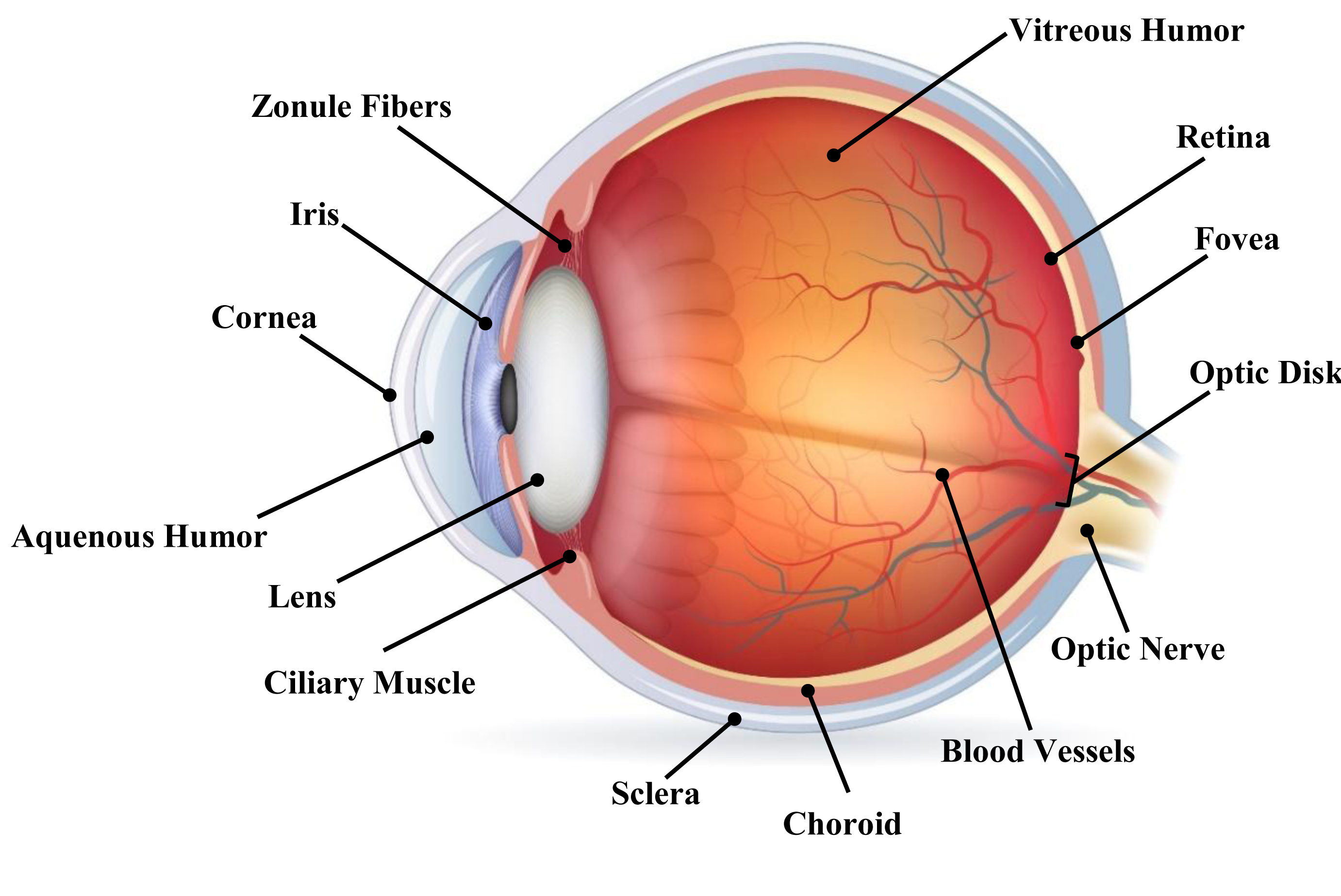
Figure 1 illustrates a structure of the human eye. A beam of light, having passed through the cornea, which has the image to an extent focused, passes through the anterior chamber, the pupil, and then the lens, which enhances the image further. The retina is supported by its retinal pigment epithelium, being typically opaque, the choroid and also the sclera.³²

Figure 1 Structure of the human eye.³⁰

Additionally, Figure 1 epitomizes a side view of the eye. The retina thickness is close to $\frac{1}{2}$ mm, and it covers $\frac{4}{5}$ of the posterior and inner side of the eye. Blood vessels are of continuous patterns with little curvature, branch from the optic disk (OD), a circular similar to an oval white area measuring approximately 2×1.5mm across (about $\frac{1}{30}$ of the retina diameter). 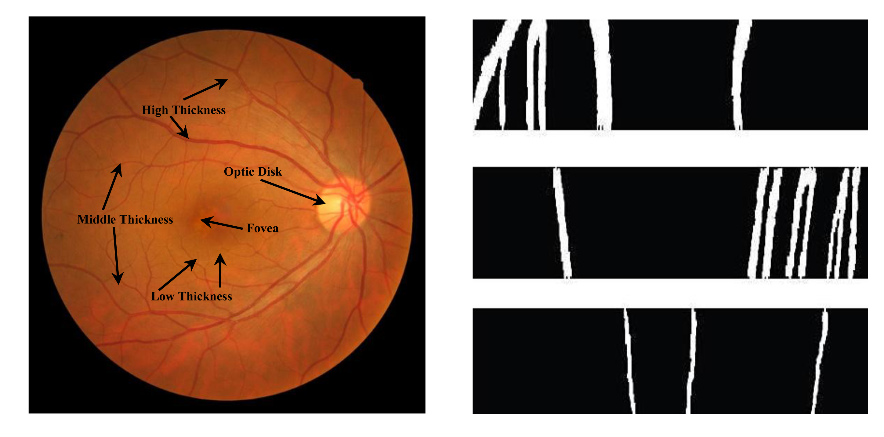The mean diameter of the vessels is close to 100μm ($\frac{1}{40}$ of retina diameter).³² Blood vessels possess continuous patterns with a slight curvature, branch from OD and are tree-shaped on the surface of the retina (Figure 2(a)).

Each person in the world has a unique blood vessels pattern. This uniqueness of the blood vessels in the retina has been widely used for biometric identification with increasing popularity. Owing to its internal location, retina is well protected against variations which might be caused by exposure to an external environment.

The vascular structure of the retina is comprised two types of vessels-arteries and veins. In comparison with veins, arteries are considerably thinner, possess a lighter red appearance and display a relatively clearer visible central light-reflex. Where the artery originates, it has a caliber of 0.1mm and further branches out on the retina initially into a main arch and subsequently into several segments. As the spreading builds up, the vessels get to be more slender to the point, which they are essentially imperceptible as capillaries. 

Finally, with respect to the size and width of the many blood vessels, doctors have classified these vessels in three main orders: The first order includes vessels with high thickness (arteries and veins) constituting the low frequency pattern in image, the second order encompasses vessels with middle thickness, making up the center frequency pattern in image, and the third order which include contents of capillaries, there exist vessels with low thickness comprising the high frequency pattern in the image. Thus, multi-resolution Contourlet method should make an appropriate method for retina blood vessels analysis. 

Being a powerful tool of multi-resolution analysis, Contourlet is capable of decomposing the image in more than one direction at different resolutions (scales). Figure 2(a) depicts the prototype of retinal image and Figure 2(b) shows the vessels in the three different orders as was mentioned above.

Figure 2 Retinal image structure. (a) A prototype retinal Image (b) High thickness vessels (up), Middle thickness vessels (middle), Low thickness vessels (down), given by wavelet transform.³⁰

Qualities and shortcomings of retinal identification 

Retinal Identification has its own particular arrangement of benefits and faults, much the same as some other kind of biometric innovation. The benefits can be depicted as takes after:³³

1. The vein map of the retina scarcely ever changes amid a human’s life range.
2.  Being located inside the eye, the retina is not exposed to (threats posed by) external environment while other biometrics, such as fingerprints, hand geometry, etc., have the potential exposure and risk of being altered.
3. The size of the actual template is substantially small by any standards. Accordingly, processing times associated with verification and identification are much shorter.
4. The rich, especial structure of the blood vessel pattern on the retina permits extraction of numerous features.
5. Retinal identification is viewed highly reliable since no two people have an identical retinal pattern

The demerits can be described as follows:

1. Retina vasculature might be afflicted by an eye disease such as cataracts, glaucoma, etc., which, if occurred can well complicate the identification process.
2. Retinal scanning technology cannot encompass bespectacled people (which require removing their glasses prior to scanning).
3. User unease as to the requirement of positioning the eye in close proximity of the scanner lens.

System architecture 

Figure 3 shows different parts of our intended biometric retinal identification. As can be seen in the block diagram, our system is comprised three main modules, namely preprocessing, proposed methodology, and feature matching. Preprocessing module includes three sub-modules: (i) rotation compensation (ii) localization of the optic disc (iii) ROI identification. Proposed methodology module is composed of (i) contourlet transform and (ii) feature extraction. Feature matching module contains the two sub-modules: (i) Mahalanobis distance (ii) similarity scores.

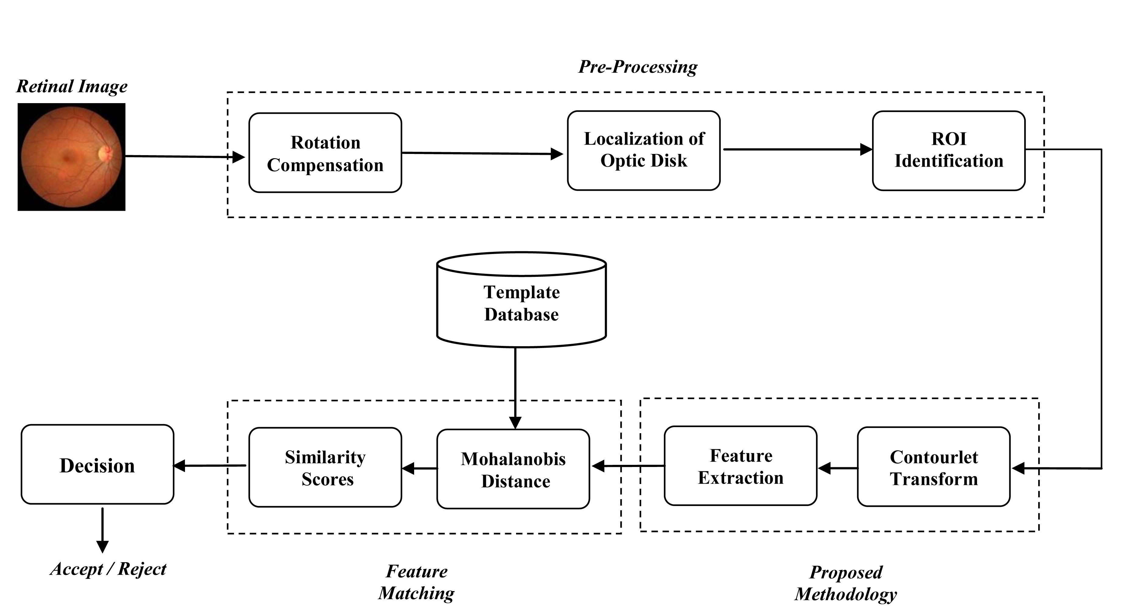
Figure 3 Block diagram of proposed method.

Rotation compensation using radial tchebichef moments

The major problem associated with using retinal images for identification arises from the inherent possibility of the eye moving in front of the fundus camera, resulting in having two different images coming from one person. This deficiency can be surmounted using a method based on the Radial Tchebichef moments, which allows estimating the rotation angle of either head or eye movement. This plan utilizes the region and the greatest radial distance of a pattern to normalize the radial Tchebichef moments.

Tchebichef moments were first appeared in a paper by Mukundan et al.,³⁴ They utilized the discrete orthogonal Tchebichef polynomials to yield a set of orthogonal moments. Where N is a positive integer, the Tchebichef polynomial of order p can be obtained by the following recurrence expression:³⁴

${\text{t}}_{\text{p}}\left(x\right)= \frac{\left\{\left(2p-1\right){\text{ t}}_1\left(x\right) {\text{t}}_{\text{p}-1}\left(x\right)\right\}-\left\{\left(p-1\right)\left(1-\frac{{\left(p-1\right)}^2}{N^2}{\text{t}}_{\text{n}-2}\left(x\right)\right)\right\} }{p}. \left(1\right)$

The initial conditions are as follows:

$t_0\left(x\right)=1 \left(2\right)$

$t_1\left(x\right)= \frac{\left(2x+1-N\right)}{N} \left(3\right)$

The Tchebichef moment with order p and repetition q and (N$\times$ M) image intensity function is defined as:²²

$T_{pq}= \frac{1}{\rho \left(p,N\right). \rho \left(p,M\right)} {\displaystyle \sum }_{x=0}^{N-1}{\displaystyle \sum }_{y=0}^{M-1}{t}_p\left(x\right) t_q\left(x\right)f\left(x,y\right) \left(4\right)$

where p, = 0, 1,…, N – 1 and q=0, 1,…,M. The Tchebichef polynomial satisfies the condition of orthogonally with:

$\rho \left(p,N\right)= \frac{N\left(1-\frac{1}{N^2}\right)\left(1-\frac{2^2}{N^2}\right)\dots \left(1-\frac{p^2}{N^2}\right)}{2p+1}. \left(5\right)$

The moments which are defined in Eq. 4 are rotation-variant. As such, a rotation invariant approach based on the Radial Tchebichef Moments is employed so that the rotation angle of head or eye movement can be estimated.³⁵

The simple elements of Spiral Tchebichef minutes are in the actuality results of one-dimensional Tchebichef polynomials³⁴ in radial distance r and round elements of the point θ. For an image of a given size, a discrete domain for these functions is required. It is said that the most suitable mathematical structure for calculating radial Tchebichef moments entails a set of concentric rings, each defining to a steady number estimation of radial distance r from the focal point of the picture. The angle of rotation,$\alpha$ , in this method, is estimated based on the relationship which exist between the rotated and non-rotated radial Tchebichef moments.³⁵ Denoting the image intensity value at location (r,θ) as f(r,θ), the radial Tchebichef moments of the non-rotated image,$S_{pq}$ , of order p and repetition q are considering as:

$S_{pq}= \frac{1}{n . \rho \left(p,m\right)} {\displaystyle \sum }_{r=0}^{m-1}{\displaystyle \sum }_{\theta =0}^{n-1}{t}_p\left(r\right) e^{-jq\theta } f\left(r,\theta \right) \left(6\right)$

where $t_p(r)$ the p is order scaled discrete orthogonal Tchebichef polynomial, n represents the maximum number of pixels along the circumference of the circle, and m stands for the number of samples in the radial direction and the radial distance varies in the range of r = 0, 1, …, ( N/2) − 1. The angle θ is a real (as opposed to complex) quantity which vary between 0 and 2$\pi$ , measured in radians and is calculated by:

$\theta = \frac{2k\pi }{n}, k=0, 1, 2, \dots , \left(n-1\right), \left(7\right)$

Radial Tchebichef moments of the rotated image with angle ${\theta }_r=\theta +\alpha$ are obtained by: 

$S_{pq}^r= \frac{1}{n . \rho \left(p,m\right)} {\displaystyle \sum }_{r=0}^{m-1}{\displaystyle \sum }_{\theta =0}^{n-1}{t}_p\left(r\right) e^{-jq\left(\theta +\alpha \right)} f\left(r,\theta \right). \left(8\right)$

With consider an image which is pivoted about the starting point; origin (r = 0), by an angle α has its intensity values kept up amid rotation, the moments$S_{pq}$ can switch over to $S_{pq}^r$ , where $\alpha$ is processed from (9):

$S_{pq}^r= S_{pq} . e^{-jq\alpha }. \left(9\right)$

 Both r and θ in the above equation take on integer values. The mapping between (r, θ) and image coordinates (x, y) is governed by:

$\{\begin{array}{c}x=\frac{rN}{2\left(m-1\right)}\cos (\frac{2\pi \theta }{n})+ \frac{N}{2} \\ y=\frac{rN}{2\left(m-1\right)}\sin (\frac{2\pi \theta }{n})+ \frac{N}{2}\end{array} \left(10\right)$

By rewriting $S_{pq}$ regarding its real and imaginary segments as $S_{pq}=D_{pq}-j{F}_{pq},$ the impacts of rotation α can be invalidated by developing the accompanying invariants:

Class 1:$V_{p0}=D_{p0} \left(11\right)$

Class 2:$V_{pq}=\sqrt{D^2{}_{pq}+ F^2{}_{pq}} \left(12\right)$

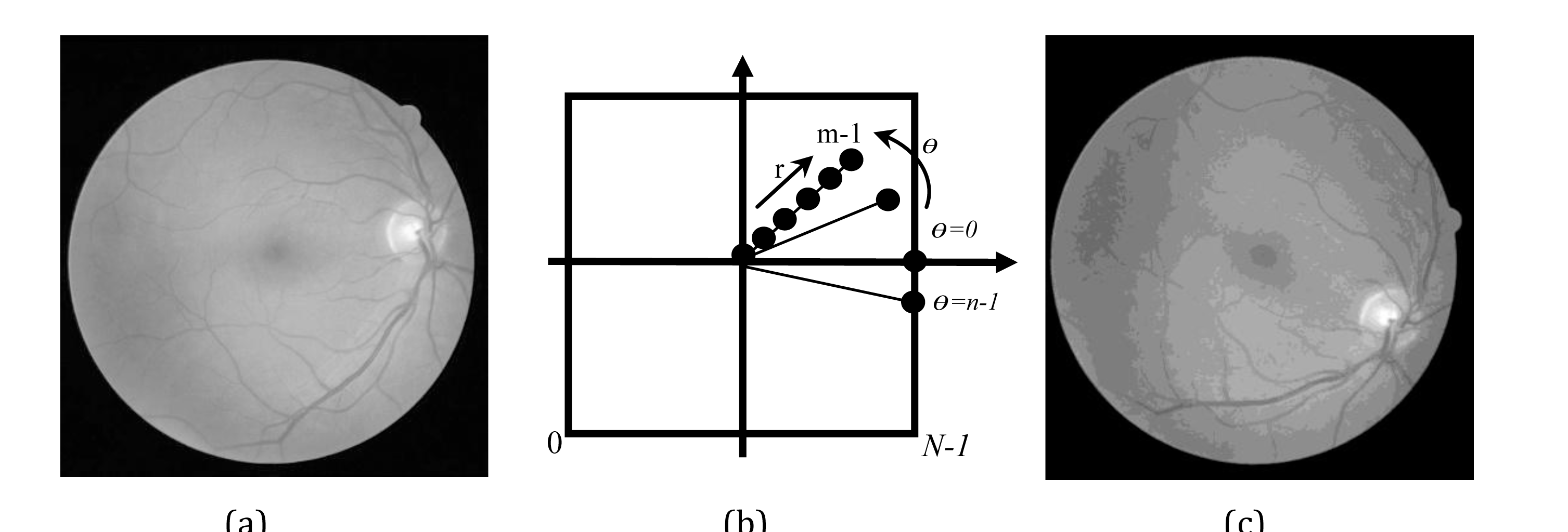
Figure 4(a) portraits the typical rotated retinal image, Figure 4(b) depicts the discrete pixel sampling of radial Tchebichef moments in polar Form and Figure 4(c) illustrates the rotation compensation associated with the right eye retinal image. Customarily “m” has an amount, which is at minimum N/2, and “n” is at 360 when the picture is sampled at single degree intervals.

Figure 4 (a) A typical rotated retinal image, (b) Tthe discrete pixel sampling of radial tchebichef moments in polar form, (c) Rotation compensation retinal image of (a).

Scale invariants of radial tchebichef moments

The magnitudes of the$S_{pq}$ are rotation invariant. Be that as it may, they are not scale or translation invariant, which is something that must be accomplished by moving the starting point to the focal point of the picture by method of centralized moments. In addition, scale invariance is achieved Scale invariant might be accomplished by scaling the primary shape to a foreordained size through calculating the zero-order moment (p=q=0), which is obtained using Eq. 13 as follows:

$S_{00}= \frac{1}{n . \rho \left(p,m\right)} {\displaystyle \sum }_{r=0}^{m-1}{\displaystyle \sum }_{\theta =0}^{n-1}{t}_0\left(r\right) e^{-j0\theta } f\left(r,\theta \right). \left(13\right)$

Then, we can obtain:

$S_{00}= \frac{1}{n . m} {\displaystyle \sum }_{r=0}^{m-1}{\displaystyle \sum }_{\theta =0}^{n-1}f\left(r,\theta \right)= \frac{A}{n . m}. \left(14\right)$

where:

A: the area of the object

m: the maximum radial distance

n: the maximum resolution used in the angular direction, which is equal to 360.

Partitioning the magnitude of the Tchebichef moments by$S_{00}$ makes every one of the moments scaled in light of the area and the greatest radials distance, the two parameters that are influenced by scaling of a shape. Accordingly, the scaled radial Tchebichef moments are determined as follows:

${Ś}_{pq}= \frac{\left|S_{pq}\right|}{S_{00}}. \left(15\right)$

In this regard, Table 1 demonstrates a prototype of a retinal image with various scaling factors (β), and what’s more, the relating magnitudes of the Tchebichef moments normalized utilizing the proposed scaling plan. As it can be concluded from Table 1 that the amounts of the relating normalized magnitudes of the Tchebichef moments persist practically unaltered under various scaling variable.

This advancement of our proposed plan normalizes is because of the way that the moments sans normalizing the pattern to a prototype size, which regularly prompts an adjustment in a few attributes of the pattern. Additionally, the proposed scaling plan is not relying on the order of the moments, and thus, the dynamic range among invariant moments is little. 

Localization of optic disc based on template matching

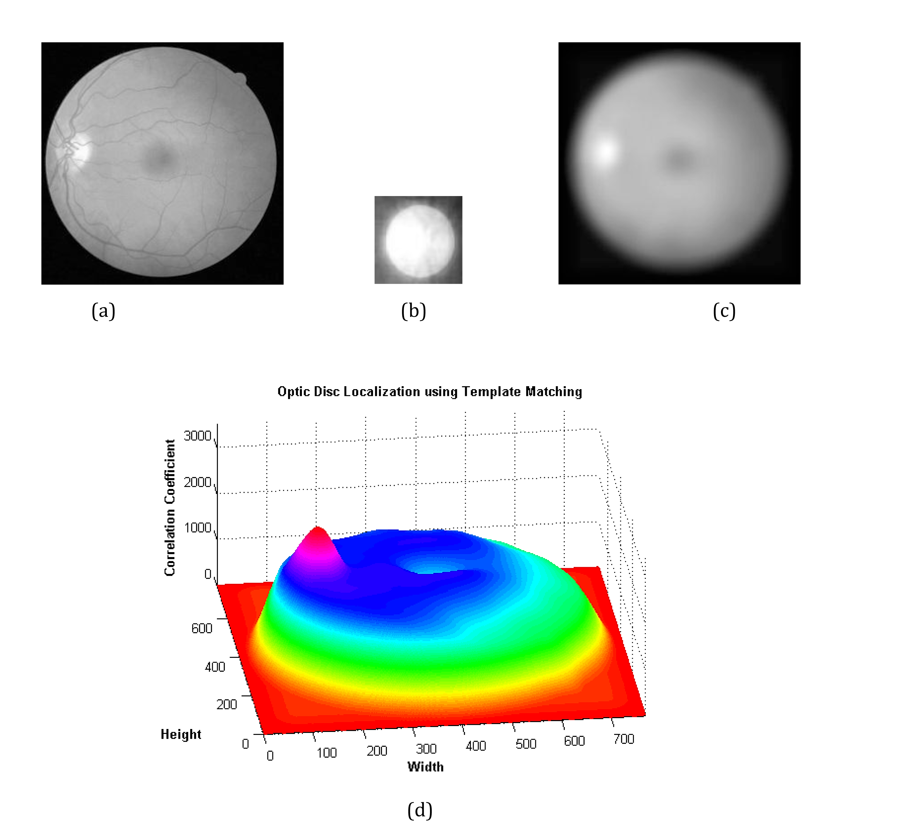
Template Matching is a popular technique, which is used to isolate certain features in an image. The execution includes a correlation of primary image and an appropriately picked template.³⁶ The most apt match is then localized based upon some criterion of optimality. Regarding the size of the optical plate local in our retinal dataset images, we made a 68 × 68 pixels template picture by taking an average over the optic plate local in 25 retinal images, each chose from our image dataset (Figure 5(b)). 

This was performed by using of grey levels exclusively owing to the fact that the result is computationally less expensive and possesses sufficient accuracy. The normalized Correlation Coefficient (CC) has the following definition:

$R\left(i,j\right)= \frac{{{\displaystyle \sum }}_k{{\displaystyle \sum }}_l \left(f_{k+i, l+j}- \overline{f_{i,j}} \right) \left(t_{k,l}- \overline{t} \right)}{{\left\{\left({{\displaystyle \sum }}_k{{\displaystyle \sum }}_l \left(f_{k+i, l+j}- \overline{f_{i,j}} \right){ }^2\right) {\left({{\displaystyle \sum }}_k{{\displaystyle \sum }}_l t_{k,l}-\overline{t} \right)}^2 \right\}}^{0.5}} \left(16\right)$

where f and t denote the original image and the template respectively, $\overline{t}$ represents the template pixels mean value; likewise $\overline{f}$ represents the image pixels mean value in the region, and is defined by the template location. 

Here, for every retinal image we quantified the normalized correlation coefficients to give a sign of how much the template picture and every individual pixel in the picture under study are coordinated. Figure 5(a) and 5(c) demonstrate a typical retinal image along with its evaluated normalized CC values.

As can be seen, the optic disc region is highlighted for distinction. The optic disc pixels represent the area with the acme of matching, thereby providing the highest CC values. The highest matched point is displayed as the brightest point in the correlation image (Figure 5(d)). We assume this point’s coordinates as a viable candidate for the location of the optic disc center.

Figure 5 Localization of optic disc based on template matching. (a) A typical retinal image, (b) Close up view of the template image (c), Correlated image, (d) Correlation coefficients (CC) values.

In fact, this technique has a propensity to locate the optic disc center to some extent toward the temporal side, which is majorly due to the asymmetric nature the optic disc carries. The reference point (CC) is required to obtain ROI identification so that explanation in the next step. In this paper, we have chosen this point as the maximum value of 3D image and have based the decision-making upon that.

Region of interest (ROI) identification

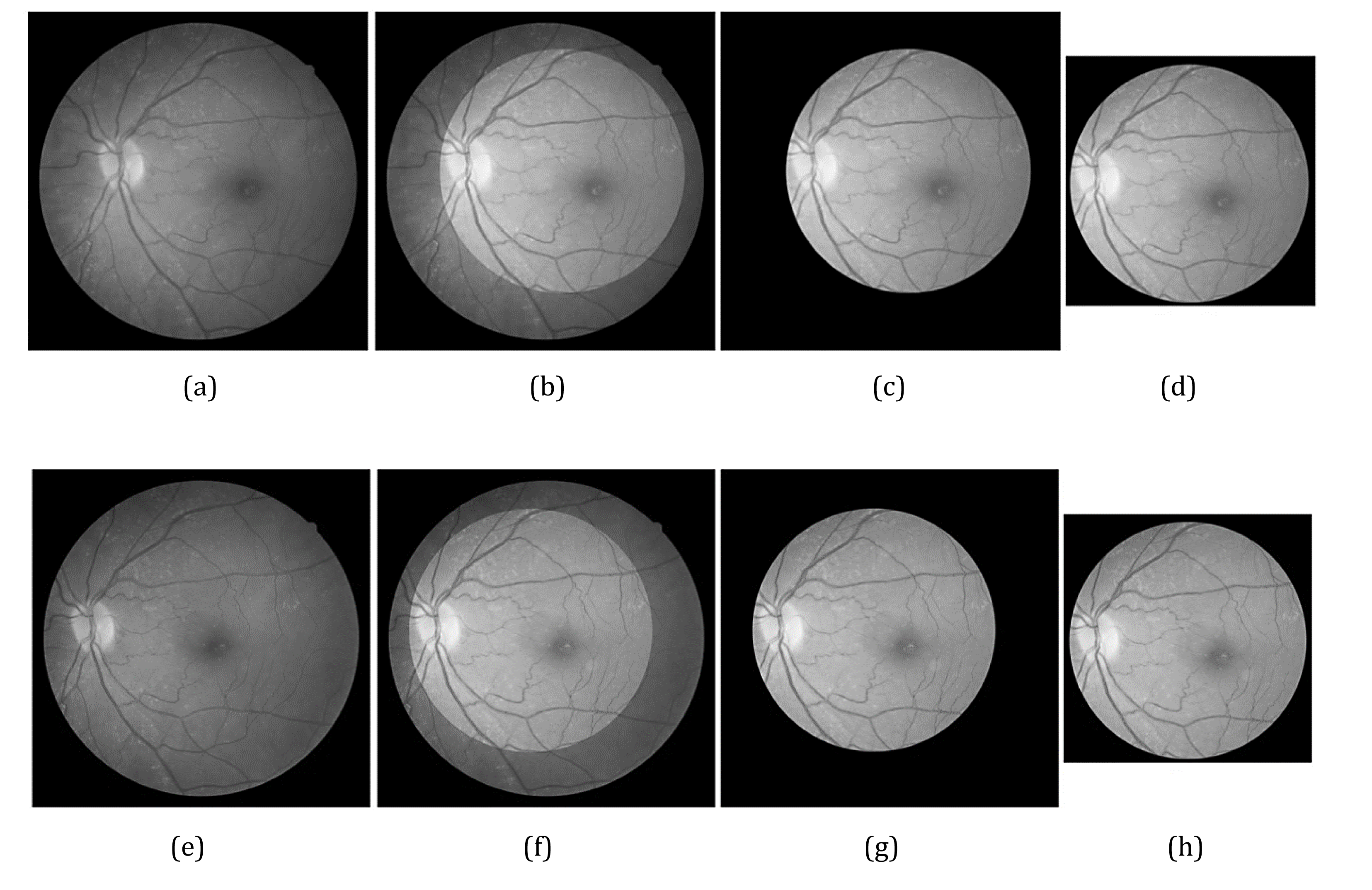
The involuntary eyeball movements in the scanning process can potentially produce different images taken from the same individual, which means that some parts of the first image may not be present in the second image and vice versa. To obviate this  disadvantage and eliminate the background from images, we are to find Region of Interest (ROI). In Figure 6, two different retinal-image samples from the same person in our database are illustrated.

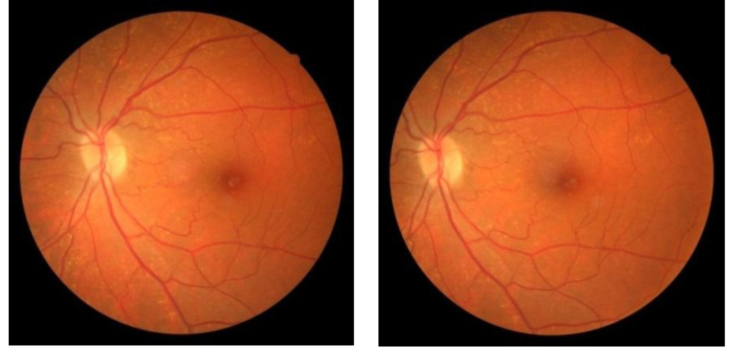
Figure 6 Two different samples of retinal images from same person in our database.

ROI identification is achieving as followed:

step1: Color retinal fundus image is converting into a gray image from the green channel.

step2: Rotation compensation and scale or translation invariant of retinal image.

step3: Find the optic disc with template matching algorithm.

step4: Compute the reference point (CC) in optic disc.

step5: At a distance of 50 pixels from the reference point (CC) in optic disc, a circle area (search space) with 500 pixels diameter in order to extract ROI was drawn. The final size of each image is 512×512. The ROI area consists of common points in both different images of the same person.

The contourlet transform

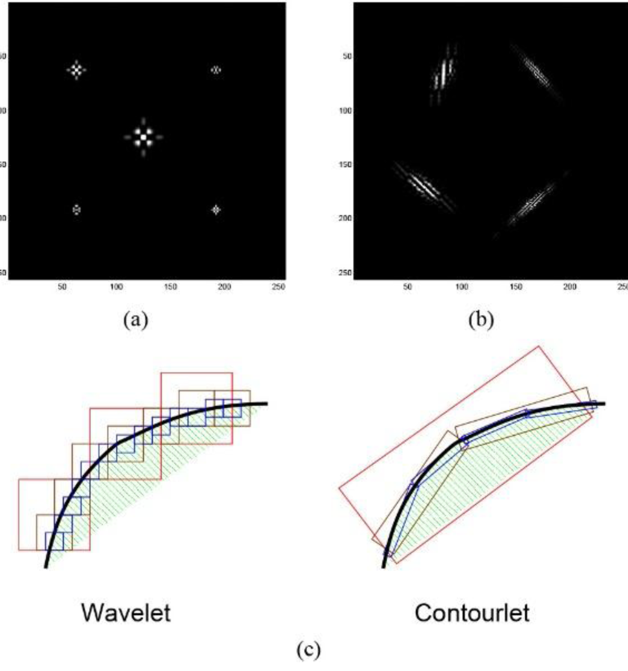
The main goal of the contourlet construction^37,38 was to acquire a sparse expansion for typical images which are piecewise smooth away from smooth contours. Wavelets of two dimensions, with tensor-product basis functions, as shown in Figure 8(a), lack directionality and are only effective in capturing point discontinuities, and fail to capture the geometrical smoothness of the contours.

Candes and Donoho³⁹ developed a new multi-scale transform, calling it the curvelet transform. The transform possessed some key features such as the high directionality and anisotropy. However, being defined in the frequency domain, it is not clear how curvelets are actually sampled in the spatial domain. A filter bank structure was proposed that can effectively deal with piecewise smooth images with smooth contours. The consequent image expansion is a frame consisting of contour segments, and hence the name contourlet was suggested.

Figure 7 ROI identification in two various images of the same person. (a), (e) original images, (b), (f) suitable ROI, (c), (g) ROI obtained based on the proposed method, (d), (h) final image after ROI identification.

Contourlet transform yields a flexible image with multi-resolution presentation. In comparison with wavelet and curvelet, contourlet results in richer directions and shapes, whereas 2D wavelet transform is only capable of capturing data in horizontal, vertical and diagonal directions. Moreover, contourlet transform displays a higher performance when it comes to depicting the geometrical structure of images. Passing through contourlet transform, the low frequency sub-images are supplied with a large amount of energy and as a result, they suffer slight impact caused by regular image processing. The outcome about transform not just has the multiscale and time-recurrence confinement means connected with wavelets, however, offers a high-level of directionality and anisotropy too.

The contourlet transform when compared to multi-scale or directional image representations transform demonstrate three principal advantages as followed:^s                       

1. Multi-resolution: Regardless of the resolution level, images are allowed to be successively approximated by the representation provided.
2. Directionality: The representation includes basis elements oriented in a variety of directions, significantly more than the few directions offered by separable wavelets.
3. Anisotropy: Representation consisting basis elements which incorporate a variety of elongated shapes with different aspect ratios leads to capturing smooth contours in images.

In particular, contourlet transform includes basis functions which are oriented at any power of two’s number of directions permitting flexible aspect ratios; some examples are shown in Figure 8(b). Benefiting from such a rich set of basis functions, contourlets can provide a smoother contour with less number of coefficients when compared with wavelet, as illustrated in Figure 8(c). 

Figure 8 Contourlet and wavelet representations for images. (a) Examples of five 2D wavelet basis images, (b) Examples of four contourlet basis images, (c) Outline indicating how wavelets having square backings can just catch point discontinuities, though contourlets having stretched backings can catch capture linear segments of contours, what’s more, in this way adequately create a smooth contour with less coefficients.³⁶

The laplacian pyramid: The primary principle of contourlet transform is initiated by using a wavelet-like multi-scale decomposition which captures singular values of the edge, after which the neighboring singular values are assembled into the contour segment. Laplacian pyramid (LP) is employed to perform a multi-resolution decomposition throughout the image to capture the singular points. Illustrated in Figure 9, this decomposition process includes “H” and “G” modules, (lowpass) analysis and synthesis filters, respectively; M represents the sampling matrix.⁴⁰ The LP decomposition within each level creates a down sampled low-pass version of the original and the discrepancy between the original and the prediction, which results in a bandpass image.

Figure 9 Laplacian pyramid. (a) One level of decomposition, the yields are a coarse guess and distinction b between the primary signal and the expectation, (b) The new recreation plan for the laplacian pyramid.³⁸

It is basic with low computational intricacy because of its single filtering channel and has greater dimension. LP is a multi-scale division of the $L^2\left(A^2\right)$ space into a progression of expanding by:

$L^2\left(A^2\right)= V_{m_o} \oplus {\displaystyle \sum }_{m=m_0}^w\left(W_m\right) \left(17\right)$

where $V_{m_o}$ is the approximation at scale$2^m$ and multi-resolution$W_m$ contains the added detail to the finer scale$2^{m-1}$ . By utilizing L low pass filters that are approximated, L low pass estimate of the picture is developed. The contrast between every estimate and its taking after down sampled lowpass adaptation adds up to a bandpass picture. A Laplacian pyramid with L+1 equal-size levels is the result, which includes coarse image approximation and L bandpass images.

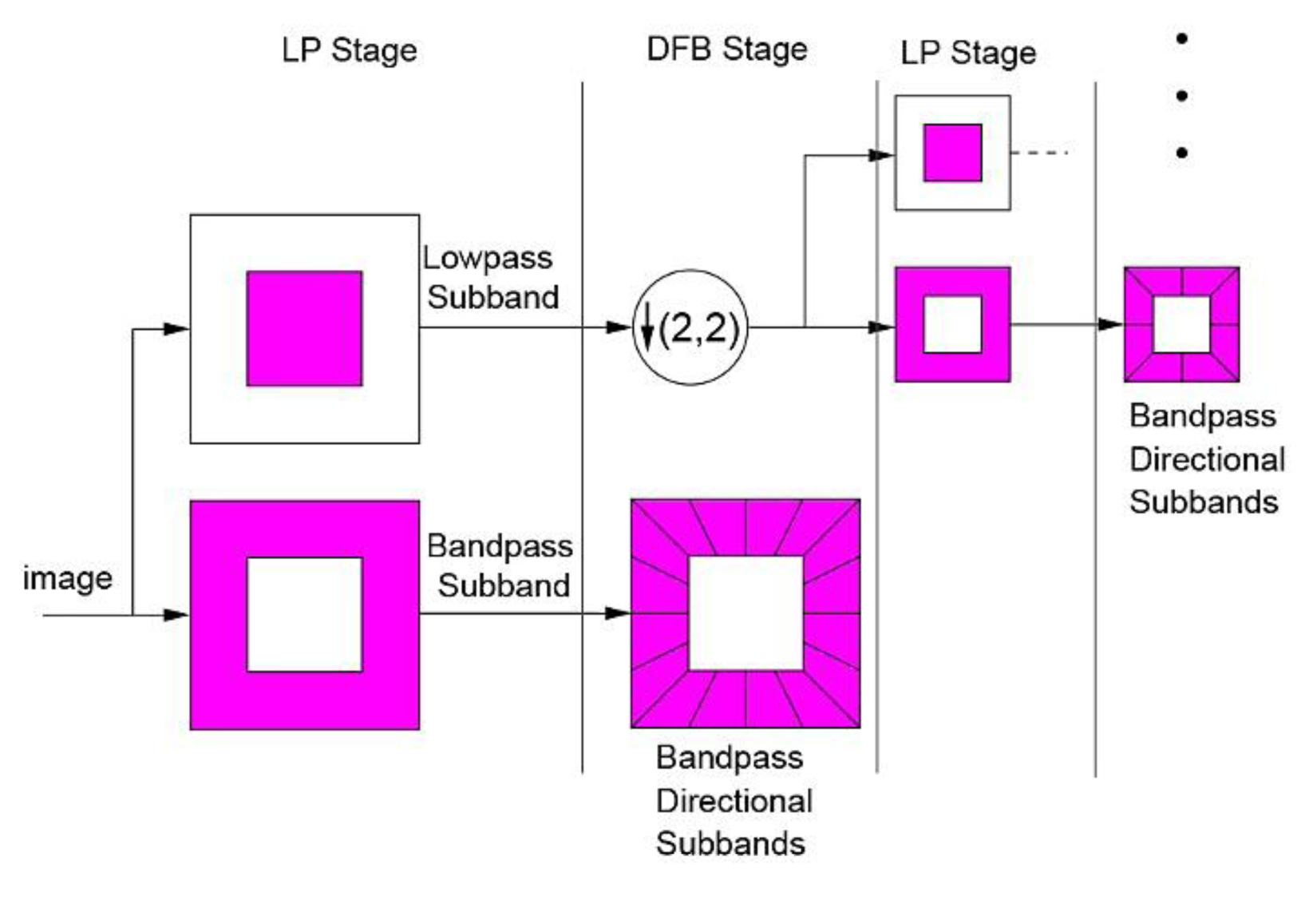
Directional filter bank (DFB): It is utilized to associate these point discontinuities and build up linear structures. As can be seen in Figure 10, DFB has the task of dividing the highpass image into directional subbands as well as showing a multi-resolution and directional decomposition of the contourlet filter bank, which is comprised an LP and a DFB. Directional information is obtained by having bandpass images from the LP fed into DFB.⁴¹ 

Figure 10 The scheme of contourlet filter bank: basically, a multi-scale decomposition into octave groups of the laplacian pyramid is figured, and afterward a directional filter bank is connected to each bandpass channel.³⁹

The fundamental function of the DFB involves using an appropriate combination of shearing operators in conjunction with two-directional partition of quincunx filter banks positioned at each node in a binary tree-structured filter bank so that the desired 2D spectrum division can be achieved, as shown in Figure 11.

Figure 11 Directional filter bank. (a) The DFB frequency response decomposition in three levels, (b) One case of the vertical DFB with three levels, (c) One case of the horizontal DFB with three levels.³⁹

It can be seen from the Figureure that in vertical DFB and horizontal DFB, generally vertical directions can be gotten (directions among${45}^{°}$ and ${135}^{°}$ ) and significantly horizontal directions (directions among$- {45}^{°}$ and$+{45}^{°}$ ).⁴¹

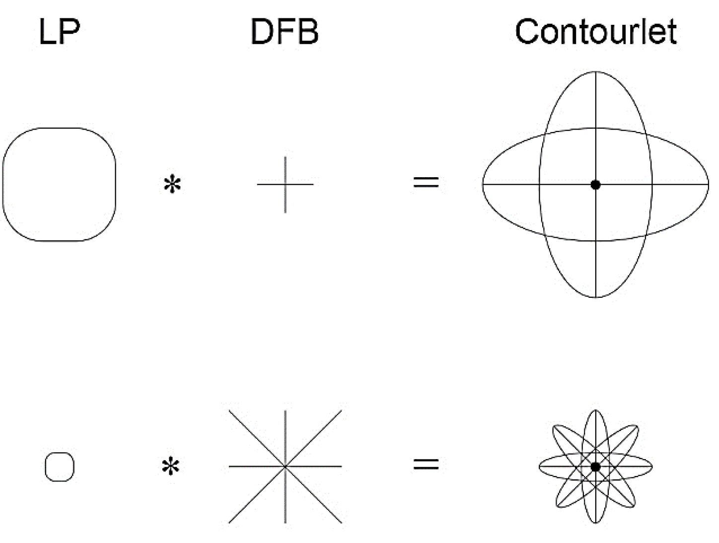
Pyramidal directional filter bank: Contourlet transform is considered as a dual filter structure, which is named pyramidal directional filter bank (PDFB). To satisfy the anisotropy scaling relation in the contourlet transform, the number of directions in the PDFB must be doubled at every other finer scale of the pyramid.³⁸ The backings of the simple functions delivered by such a PDFB are graphically shown in Figure 12. As is evident from the two illustrated pyramidal levels, the number of directions of the DFB is doubled, whereas the support size of the LP is reduced by four times. 

Figure 12 Delineation of the backings for the contourlet executed by a PDFB that fulfills the anisotropy scaling connection. from the uppermost line to the lowest line, the scale is decreased by four, at the same time the quantity of directions is multiplied.³⁶

Consolidating these two stages, the PDFB premise functions will have their support size changed starting with one level then onto the next as indicated by the curve scaling connection. In the contourlet scheme in question, each generation doubles the spatial resolution and the angular resolution. Since the PDFB supplies a frame expansion for images which consist of frame elements like contour segments, it is called the contourlet transform as well. The DFB, which is proposed here is a 2D directional filter bank allowing perfect reconstruction to be achieved. 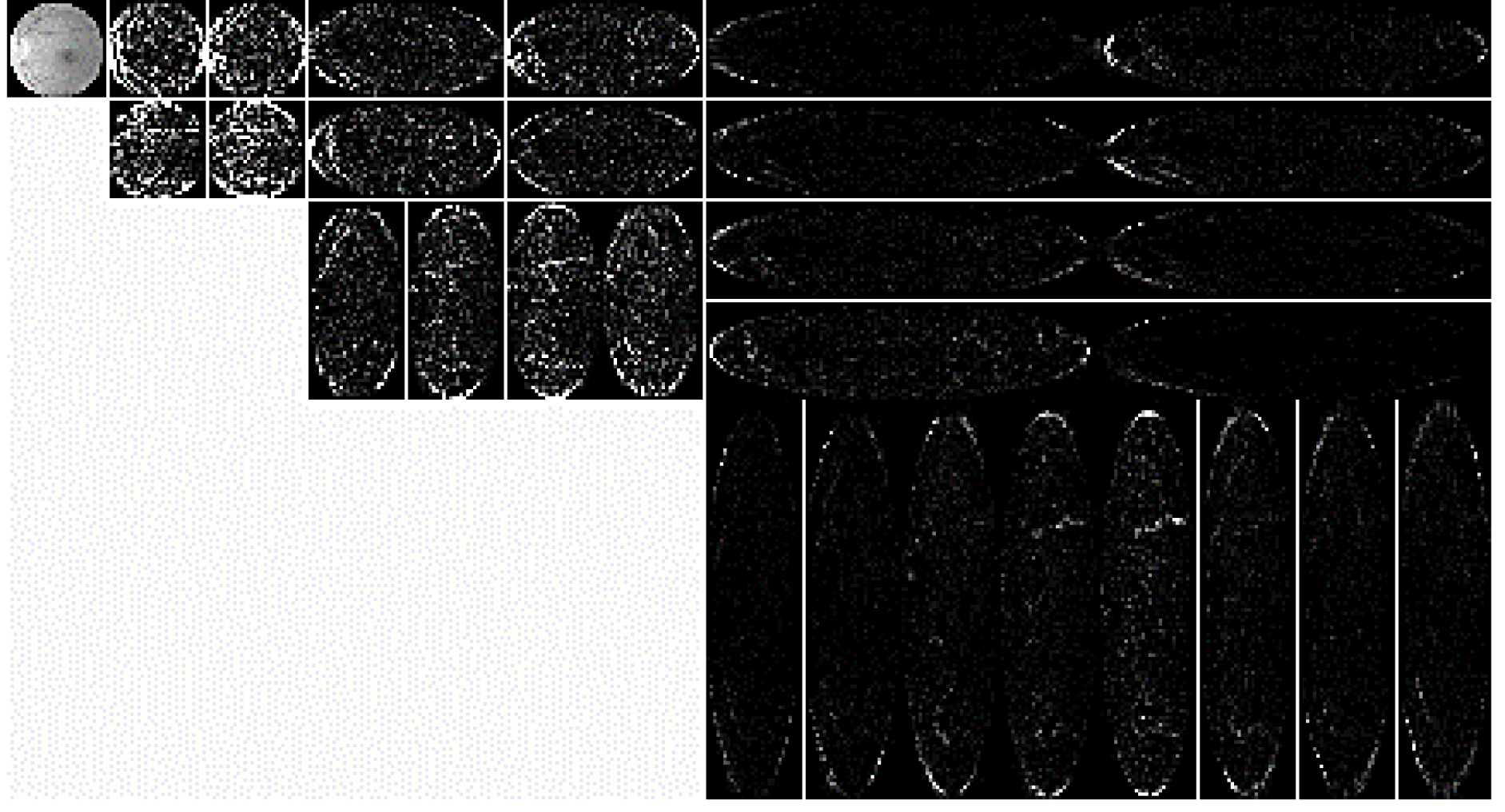The original DFB is implemented by means of m-level binary tree and results in $2^m$ subb ands with wedge-shaped frequency partitioning, “m” being the level of the directional filter.³⁸ Figure 13 illustrates the next contourlet decomposition upon a retina sub-image. To achieve visualization with a high clarity degree, each image is only decomposed into triad pyramidal levels, which are subsequently decomposed into 4, 8 and 16 directional subbands. Performing the contourlet transform on the retina provided diverse subbands, each one of which interprets the image characteristics in a particular direction.

Figure 13 Illustrations of contourlet transform of the retinal image in three pyramidal levels decomposition, which are then decomposed into 4, 8 and 16 directional subbands. little coefficients are shaded dark while huge coefficients are hued white.

 Feature extraction

Because of the iterated lowpass filtering, the texture data with higher congruity has been isolated; subsequently the texture data are mainly contained in the directional subbands of every scale. Thusly, the lowpass picture is disregarded while ascertaining the texture component vector. A set of statistical texture features introduced in literature are used in this study as an assessment criterion. This set is introduced in Table 2: Mean energy, standard deviation and information entropy are the features which are used for the contourlet space in⁴² and.⁴³

where:

$F_{mk}$ : sub-image of the k^th orientation in the m^th level of decomposition

$X_{mk}$ : row-size of the sub-image$F_{mk}$

$Y_{mk}$ : column-size of the sub-image$F_{mk}$

The energy is the prominent feature which can be employed in the textural feature extraction. In this work, the mean energy (Eq. 18) of each subband image (sub-image) is calculated. In addition, standard deviation serves to capture the scale of the diversity of the image and is defined as in (Eq. 19), while information entropy is an index representing the complexity of the texture data and is defined as in (Eq. 21). Moreover, contrast (Eq. 23) is a measure of the amount of neighborhood varieties showing in the picture, whereas homogeneity (Eq. 24) relates to the texture’s contrast. Consequently, the feature vector of the subband image $\left(R_{mk}\right)$ on the k^th direction at the m^th level is defined as:

$R_{mk}= \left\{A_{mk}, B_{mk}, C_{mk}, D_{mk}, E_{mk} \right\} \left(25\right)$

A contourlet transform decomposition which includes the picture being decomposed by a J level Laplacian pyramid decomposition with a $P_m$ sub-image directional filter bank utilized at the m^th level, ( m = 1, 2,…, M ) is alluded to as M level, for which the aggregate number of directional sub-image $P_{total}$ is ascertained as: 

$P_{total}= {\displaystyle \sum }_{m=1}^M{P}_m \left(26\right)$

By computing the feature vector of every sub-image, these vectors are then modified and joined to constitute the complete feature vector$R= \left\{A_i, B_i, C_i, D_i, E_i\right\} , i=1,2,\dots , P_{total , }$ of the entrance picture as appeared on: 

$R= \left\{A_1,\dots , A_{P_{total}},B_1,\dots , B_{P_{total}},C_1,\dots , C_{P_{total}},D_1,\dots , D_{P_{total}},E_1,\dots , E_{P_{total}} \right\} \left(27\right)$

where$A_i, B_i, C_{i },D_i and E_i$ show the corresponding statistical measure of the i^th directional sub-image of the retinal image decomposition. Here, the number of elements rises exponentially with the level of DFB decomposition. 

Matching scores based on mahalanobis distance

Feature Matching involves comparing the Feature vector, which is generated for the query image, provided in the testing phase, versus stored feature vector in the database that is obtained during the training phase. The matching phase of the retinal identification process necessitates the following steps:⁴⁴

Computing the distance d(x,z) extending between the retinal biometric template z and the real test retinal sample x;

• Performing distance score normalization;
• Converting distance to similarity-score ;
• Computing the set of similarity scores for identification (1: N).

Distance in the feature space

So as to calculate the distance score between the biometric template “z” and the current biometric test “x”, Mahalanobis distance was utilized, which is given by:⁴⁵

$d_M\left(x,z\right)= \sqrt{{\left(x-z\right)}^T . {({{\displaystyle \sum }}^{\text{}}\left(x-z\right))}^{-1} } \left(28\right)$

where $"{{\displaystyle \sum }}^{\text{}}"$ is two retinal feature vectors covariance matrix:

${{\displaystyle \sum }}^{\text{}}=cov\left(x,z\right)=E{\left[\left(x-E\left[z\right]\right).\left(x-E\left[z\right]\right)\right]}^T \left(29\right)$

The reason we chose to use this distance metric in the feature vector space was owing to its principal properties: scaling invariance and feature correlation exploiting.⁴⁵ The firstproperty is paramount specifically because the application needs to scale the features so that it can compare them against different individuals and to investigate the features contribution on the identification accuracy. The second property gains significance as it allows an earlier selecting for the optimal feature subsets, which is based on their correlation. This obviates applying more computationally expensive feature selection algorithms.

 Distance score normalization

The distance score normalization serves to provide a common value range of all matching scores which will be computed for the biometric patterns. There are numerous normalization techniques available, such as Z-Score Normalization, Decimal Scaling Normalization, Min-Max normalization, Sigmoid Normalization and so on. For our available biometric data, we opted for the double sigmoid function, given by:

$D\left(x,z\right)=\{\begin{array}{c}for d_M\left(x,z\right)<\theta : \frac{1}{1+ A_1 . \text{exp}\left[-B_1 . \left( \frac{d_M\left(x,z\right)- \theta }{C_1}\right)\right]}\\ for d_M\left(x,z\right)\ge \theta : \frac{1}{1+ A_2 . \text{exp}\left[-B_2 . \left( \frac{d_M\left(x,z\right)- \theta }{C_2}\right)\right]}\end{array}\left(30\right)$

where:

• the coefficients $A_1, A_2, B_{1 }and B_{2 }$ are attained from the experimental data; they are in fact shape parameters for the sigmoid function;
• $C_1$ and$C_{2 }$ represent the quasi-linear behavior region boundaries for the sigmoid function; these parameters are obtained from the experiment as well;
• $\theta$ is a threshold value related to the security level, which is set for the application.

The normalized distance score is acquired by measuring the difference between the test retinal feature vector “x” and the compared biometric template “z”.

Distance to similarity conversion

In order to determine the similarity or the level of matching between the current biometric sample x and the biometric template “z”, it is essential to apply an additional transform so that the highest scores would mean more similarity while the lowest scores would translate as larger difference. All the computed scores vary in the range [0,1], as governed by the property of the sigmoid function. Owing to this range, the distance-to-similarity conversion can be performed by:

$S=s\left(x,z\right)=1-D\left(x,z\right) \left(31\right)$

Set of the similarity scores

We are computing N scores for each person to be identified, the comparison being 1:N. Thus, the identification similarity scores are given by:

$S_i=\{{}_{for d_{M,i}\left(x,z_i\right)\ge \theta : \frac{ A_2 .\exp \left[-B_2 . \left( \frac{d_{M,i}\left(x,z_i\right)- \theta }{C_2}\right)\right]}{1+ A_2 .\exp \left[-B_2 . \left( \frac{d_{M,i}\left(x,z_i\right)- \theta }{C_2}\right)\right]}}^{for d_{M,i}\left(x,z_i\right)<\theta : \frac{ A_1 .\exp \left[-B_1 . \left( \frac{d_{M,i}\left(x,z_i\right)- \theta }{C_1}\right)\right]}{1+ A_1 .\exp \left[-B_1 . \left( \frac{d_{M,i}\left(x,z_i\right)- \theta }{C_1}\right)\right]}}, i=\overline{1,N} \left(32\right)$

Finally, Figure 14 shows the more detailed of our proposed methods after contourlet decomposition of the input retinal image.

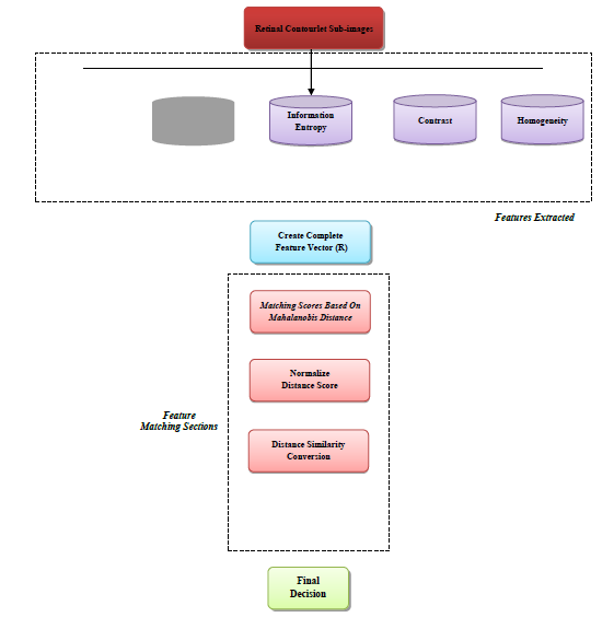
Figure 14 Our detailed proposed method after contourlet transform.

The experimental database

In this work, all our experiments were implemented in MATLAB with 4.2GHz CPU, and 8GB memory. Experiments utilized a self-built database containing 5500 retinal images taken from 550 different people (10 images with different rotations and scale ranges). In order to test and analyze of our proposed algorithm under real conditions, we used the digital fundus camera that existed in our country with “TopCop” brand, in over a time span of three years. Therefore, our self-built database permissions the framework to be tried in entirely hard conditions and recreating a more sensible and practical environment.

These retinal images were taken from people of different ages and both genders and encompass all the potential diseases which may have any tangible effect on the retinal. The diverse conditions are additionally considering the way that distinctive specialists with various contrast and illumination designs on the camera have gained the pictures. Six of these were utilized to train the template and the staying four samples were utilized for testing. In order to evaluate the robustness in terms of rotation and scale invariance, we rotated and scaled the database, respectively. 

The three rotation angles used are$\pm {15}^{°}, \pm {25}^{°}, \pm {35}^{°},$ and the scale ranges include$1\pm 0.05, 1\pm 0.10, 1\pm 0.15$ . The size of the original retinal images was 700×700 pixels. Referring to the brightest pixels, the ROI mask is calculated. Therefore, the final retinal images are resized to 512×512 pixels. Figure 15(a), and 15(b) shows some different individual’s samples of the right and left eyes from our database, respectively.

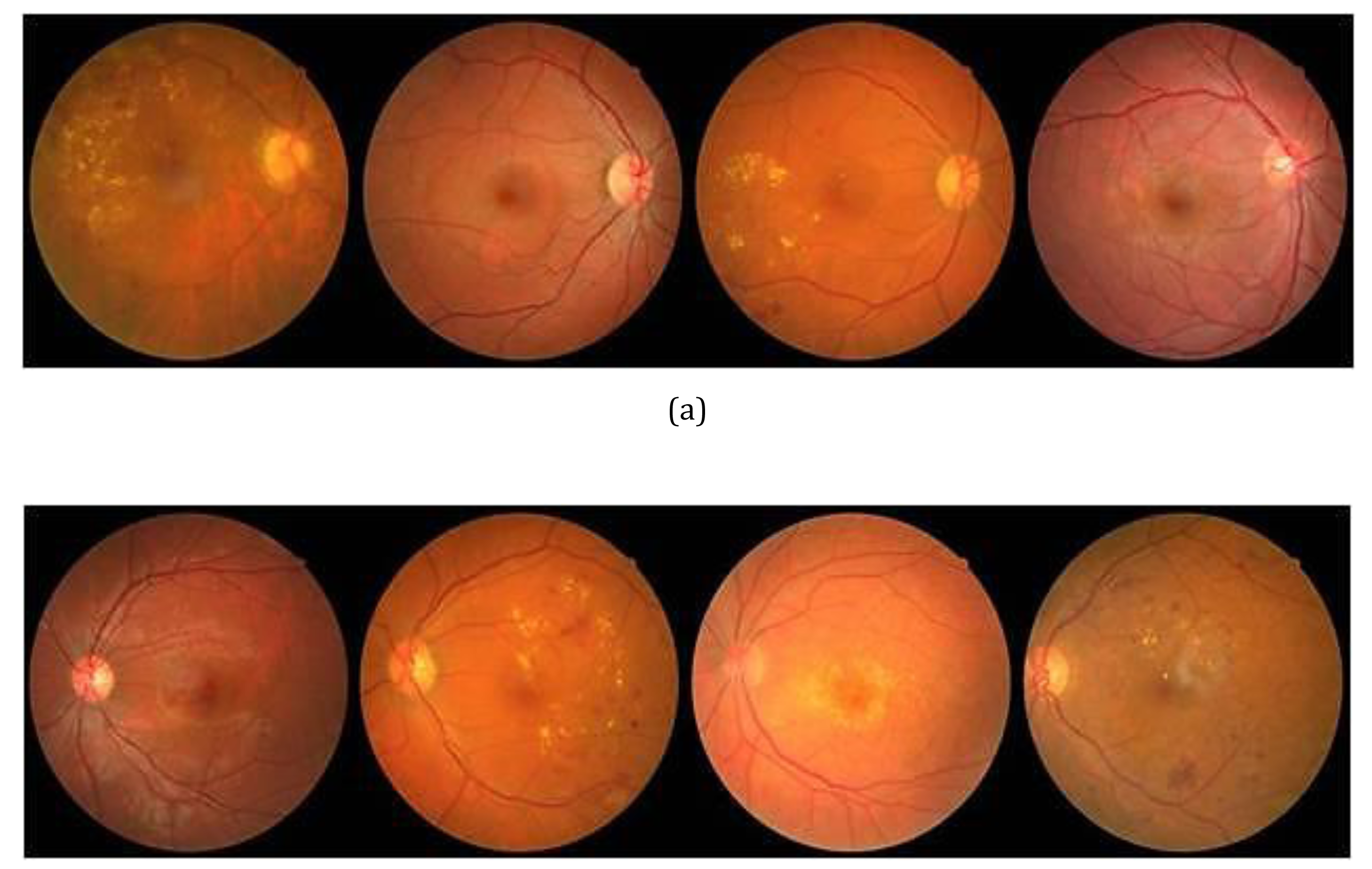
Figure 15 Some different individuals samples of our database (a) Right eyes, (b) Left eyes.

Retinal identification

Retinal identification, also called one-to-many matching, is to find an answer to the question “who is this person?” based on his/her retinal images. The genuine and imposter matching’s were employed to evaluate the most desirable level of contourlet decomposition. Within this mode, the input retina’s class is recognized, with each sample being matched against all the other samples from the same subject as well as all samples coming from the other 550 subjects. Provided the two matching samples originate from the same subject, the successful matching is called a genuine or intra-class matching. Otherwise, interclass matching or imposter is the term designated to the unsuccessful matching. 

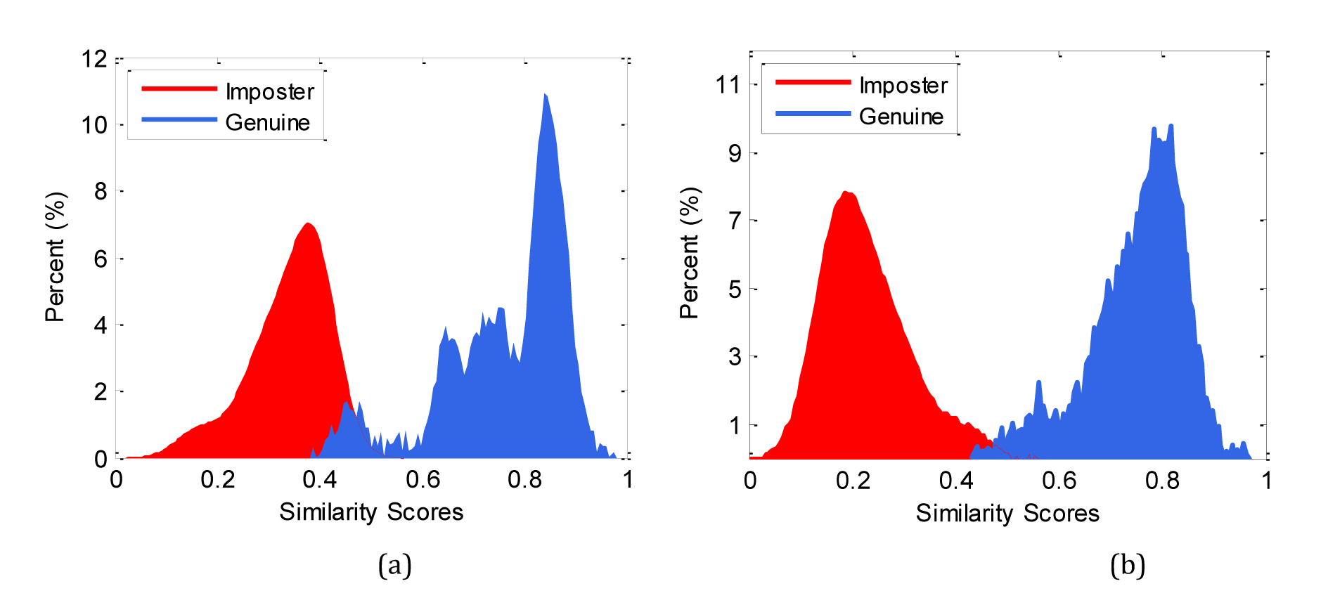
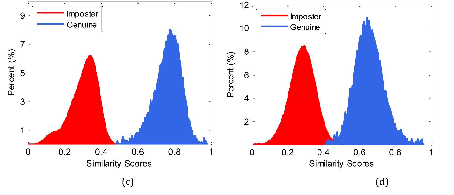
Accordingly, we make use of full matching in intraclass, where each sample is matched with all the other samples within the same class, and interclass matching, where each of the samples is matched against all the samples from the other 550 subjects. An aggregate of 1,210,000 $\left(550\times 550\times 4\right)$ matching were performed, 2,200(550 X 4)  of which accounted for genuine matchings. The genuine and imposter deliveries corresponding to the 2^nd, 3^rd, 4^th and 5^th level of contourlet transform decomposition are setup in Figure 16(a) to 16(d), respectively. As is apparent and can be seen the 4^th level of contourlet decomposition is devoid of the overlapped area; hence, this level is expected to demonstrate the highest performance in our identification system.

Figure 16 Genuine and imposter distribution of the 2nd to 5th contourlet decomposition level. (a) 2^nd level, (b) 3^rd level, (c) 4^th level, (d) 5^th level.

Biometric performance measurements criterion

Our proposed framework can be seen as a two class issues: whether a man/woman ought to assert as a genuine customer or an imposter. Keeping in mind the end goal to assess the achievement of the framework, a standard estimation is utilized to check the acceptance errors and rejection errors. They are characterized as takes after:

• False reject rate (FRR): The rate of genuine customers or approved individual that the biometric framework neglects to acknowledge. It will enlarge relatively to the security threshold. At the point when the security threshold builds, more clients (counting the approved individual) will be rejected because of the great security level. FRR is characterized as:

  $FRR=\frac{Number of rejected individual}{Overall number of individual accesses }\times 100\% \left(33\right)$

• False acceptance rate (FAR): The rate of imposters or unapproved individual that the biometric framework neglects to reject. It increases when the security threshold (matching confidence) is brought down. FAR is characterized as:

  $FAR=\frac{Number of accepted imposter }{Overral number of imposter accesses }\times 100\% \left(34\right)$

• Equal error rate (EER): Is an ideal rate where FAR is equivalent to FRR. Perceptibly, EER is perceived as the intersection point between FAR and FRR. It is normally used to decide the general accuracy of the framework.

  These three execution measures, to be specific FAR, FRR and EER will be utilized to affirm the proposed methods in the ensuing sections. In our paper, the false accept rate (FAR) versus false reject rate (FRR) is shown in Figure 17. In one-to-550 matching, all of the 2,200 (550×4) testing images were used and EER=0.0032 in 4^th level of contourlet decomposition was obtained. This Figureure is a testimony of the approach excellent performance in retinal identification.

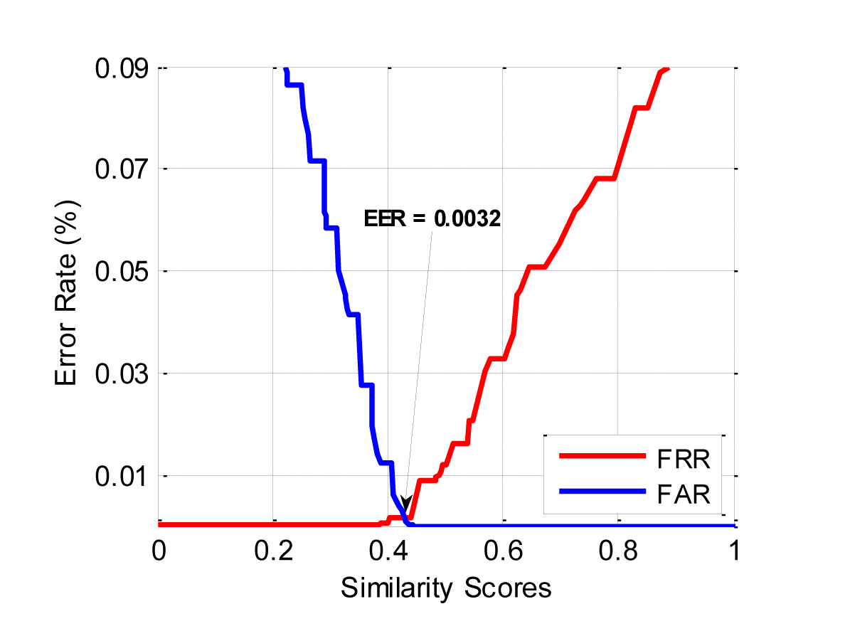
Figure 17 FAR vs. FRR curve for proposed method.

Evaluating the number of training images 

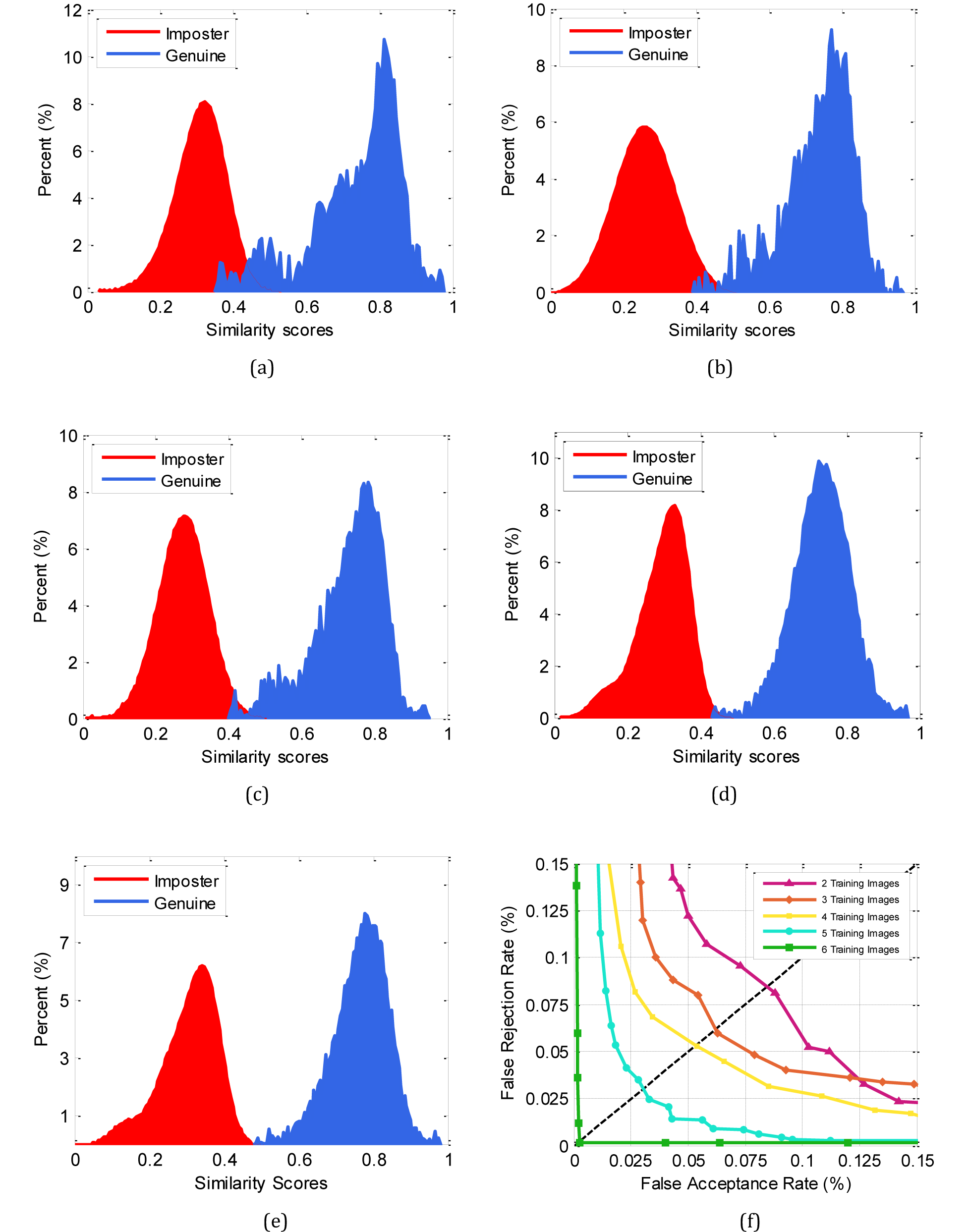
The genuine and imposter disseminations are appearing in Figure 18(a) to 18(e) while 2, 3, 4, 5 and 6 training images are utilized to train of the proposed method in 4^th level of contourlet decomposition, respectively. To reasonably represent the distinction, Figure 18(f) delineates their Receiver Operating Curve (ROC), which demonstrates the variety of the FAR FRR at various working thresholds. Additionally, the EER is utilized to quantify the framework performance that is characterized as the error rate when the FAR and the FRR are equivalent.

Figure 18 Impact of the quantity of training images on the identification accuracy utilizing: (a) By using 2 training images, (b) By using 3 training images, (c) By using 4 training images, (d) By using 5 training images, (e) By using 6 training images, (f) The receiver operating characteristics (ROC).

Table 3, demonstrates the consequences of EER from every utilizing number of training images. From these outcomes, it can be inferred that the system can work productively even with just two training images.

It can likewise be watched that utilizing five training images can give better accuracy in identification mode. This can be clarified by the way that, the utilization of more than two retinal pictures bring about more information being caught in every class. Nonetheless, utilizing more than five training images does not give further betterment.

Separability test

Decidability Index provides an excellent measure for the separability of Genuine and Imposter classes.⁴⁶ Assuming ${\mu }_G$ and${\mu }_I$ respectively denote the mean value of Genuine and Imposter Distributions, and also and represent the standard deviations of genuine${\sigma }_{G }$ and ${\sigma }_I$ imposter, respectively, we will then have the decidability $d^{\prime }$ defined as:

$d^{\prime }= \frac{\left|{\mu }_G-{\mu }_I\right|}{\sqrt{\frac{{\sigma }_G^2-{\sigma }_I^2}{2}}} \left(35\right)$

The greater the decidability record the more prominent being kept apart of genuine and imposter appropriations. The decidability indicator and all of statistical measures (i.e., means and standard deviations) in different number of training images are abridged in Table 3. The outcomes show that utilizing five and six training images in 4^th level of contourlet decomposition deliver the best division, respectively.

The rotation, scale, and ROI test

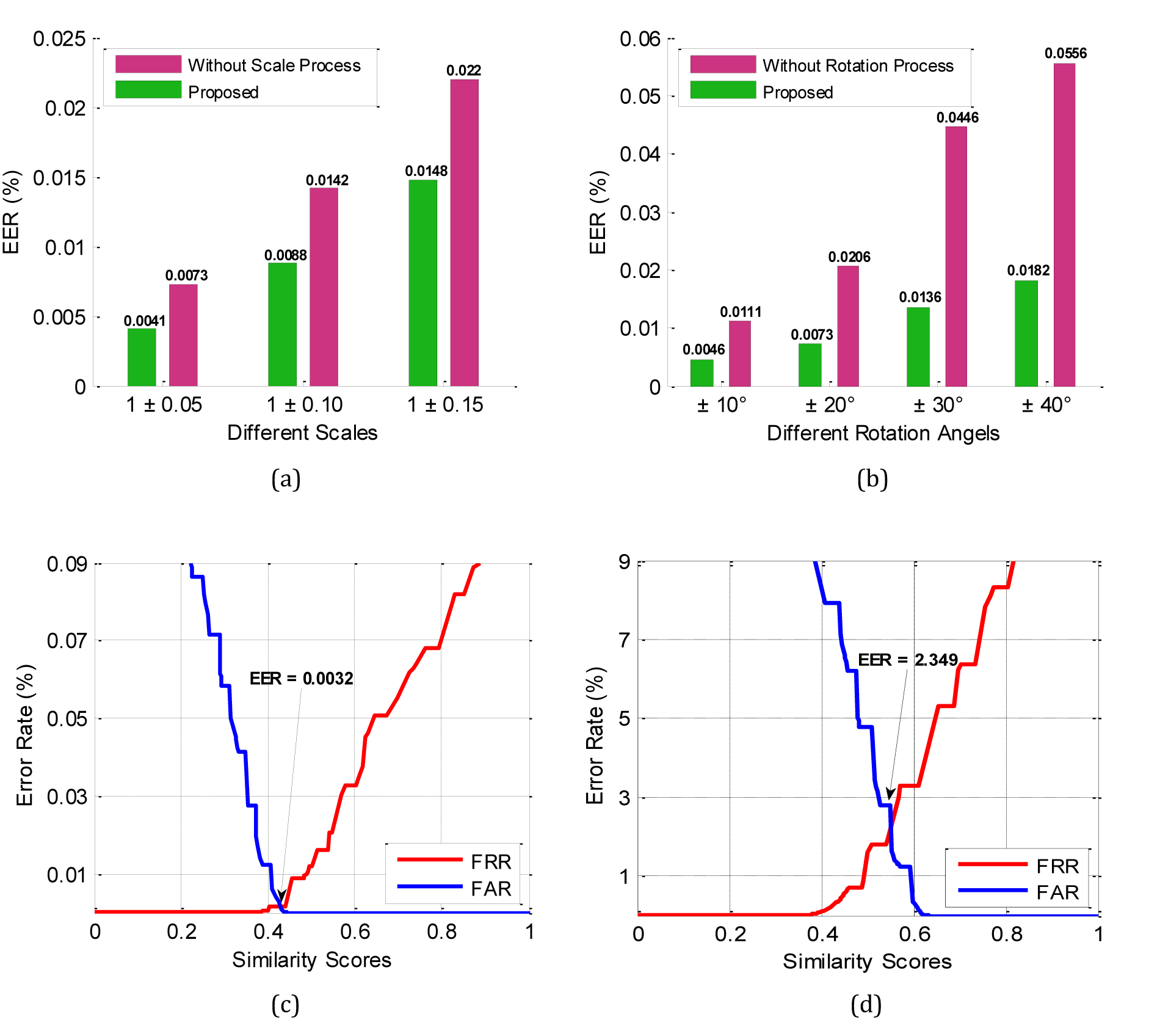
In order to the robustness to scale changes and rotations of the proposed algorithm, we lead the other check on our dataset. From the Figure 19(a), and 19(b), respectively, it can be observed that, for the proposed technique in 4^th level of contourlet decomposition, however the estimations of EER fluctuates as per scale changes or rotations, but these plots demonstrate that the proposed design structure is vigorous to scale changes and rotations. It should be note that, both rotation and scale experiments done while we have used the ROI section.

In both Figure 19(a), and 19(b), blue columns shown the EER of proposed method when we have using rotation and scale sections, while red columns shown the EER when we have not using rotation and scale sections, respectively. The sharp differences between the values of the blue and red columns in the two mentioned plots show the importance and impact of using proposed methods.

Additionally, in order to highlight the significance of the ROI method in the proposed identification system, assessment was directed by using ROI method and without using ROI method, they got aftereffects of which are graphically shown in Figure 19(c), and 19(d), respectively, so that 19(c) illustrates the FAR vs. FRR curve when the ROI method is existent and 19(d) depicts the FAR vs. FRR curve when the system is non-existent of the ROI method. Also, both Figure 19(c), and 19(d) experiments done while we have used the rotation and scale sections. Consequently, the EER value of scale, rotation, and ROI method show that the significance of these sections in our proposed method. 

Figure 19 Analyze of scale and rotation changes, and ROI evaluation. (a) EER (%) obtained difference scales, (b) EER (%) obtained in difference rotation angels, (c) Proposed identification system by using the ROI method, (d) Proposed identification system without using the ROI method.

Speed evaluation 

Table 4 records every step-time and overall-time cost of identification in proposed algorithm. Whenever there are 550 retinal templates in the dataset, the overall-time cost of identification,$T_{overall}$ , can be registered with: 

$T_{overall}=(T_{ic}+T_{rc}+T_{lop }+ T_{re}+T_{cfe}+T_{fn}+T_{fm})\times K_{template} \left(36\right)$

where:

• $T_{ia} :$ Time of image capturing 
• $T_{rc} :$ Time of rotation compensation 
• $T_{lop }:$ Time of localization of optic disc 
• $T_{re} :$ Time of ROI extraction 
• $T_{cfe} :$ Time of contourlet feature extraction 
• $T_{fn} :$ Time of feature normalization 
• $T_{fm} :$ Time of feature matching 
• $K_{template} :$ Number of template in the dataset

Performance comparison of wavelets transform vs. contourlet transform 

In this section, we assess the execution of our proposed algorithm taking into account contourlet transform, and contrasting it with Haar wavelet, Daubechies wavelet, Morlet wavelet, and Symlet wavelet. For a number of tests run, the typical ROC curves of the experimental results are illustrated in Figure 20(a). The wavelets are tested in 5^th level and the contourlet in 4^th level of decomposition. Also, Figure 20(b) shows the EER of each transforms that used in Figure 20(a). Therefore, it is evident that the properties of the coarse coefficients of contourlet are noticeably better than those of wavelets, and they achieve a high identification rate. 

Experiments on distance methods

In order to obtain superior matching, we looked at the Mahalanobis distance (proposed matching distance) with other routine distance matching methods as defined: Euclidean, Hamming, and Mahalanobis in 2^nd to 5^th contourlet transform decomposition levels in Figure 21(a) to 21(d), respectively. Furthermore, Figure 21 demonstrates the outcomes (EER) of matching methods in different number of training pictures, what’s more in different decomposition levels in our paper. Figure 21 clearly indicates that the identification performance of our proposed system (EER) for Mahalanobis distance enhances fundamentally at the point when more sample images are utilized- as a part of the training stage- as was supposed as this similarity distance, in examination with other matching methodologies. Along these lines, by expanding the training images we can gain more appropriate efficiency in proposed technique by utilizing Mahalanobis distance. 

Finally, some of state-of-the-art identification approaches together with their results are presented in Table 5. This enables researchers to conduct comparative studying with the existing works and assess their own work.

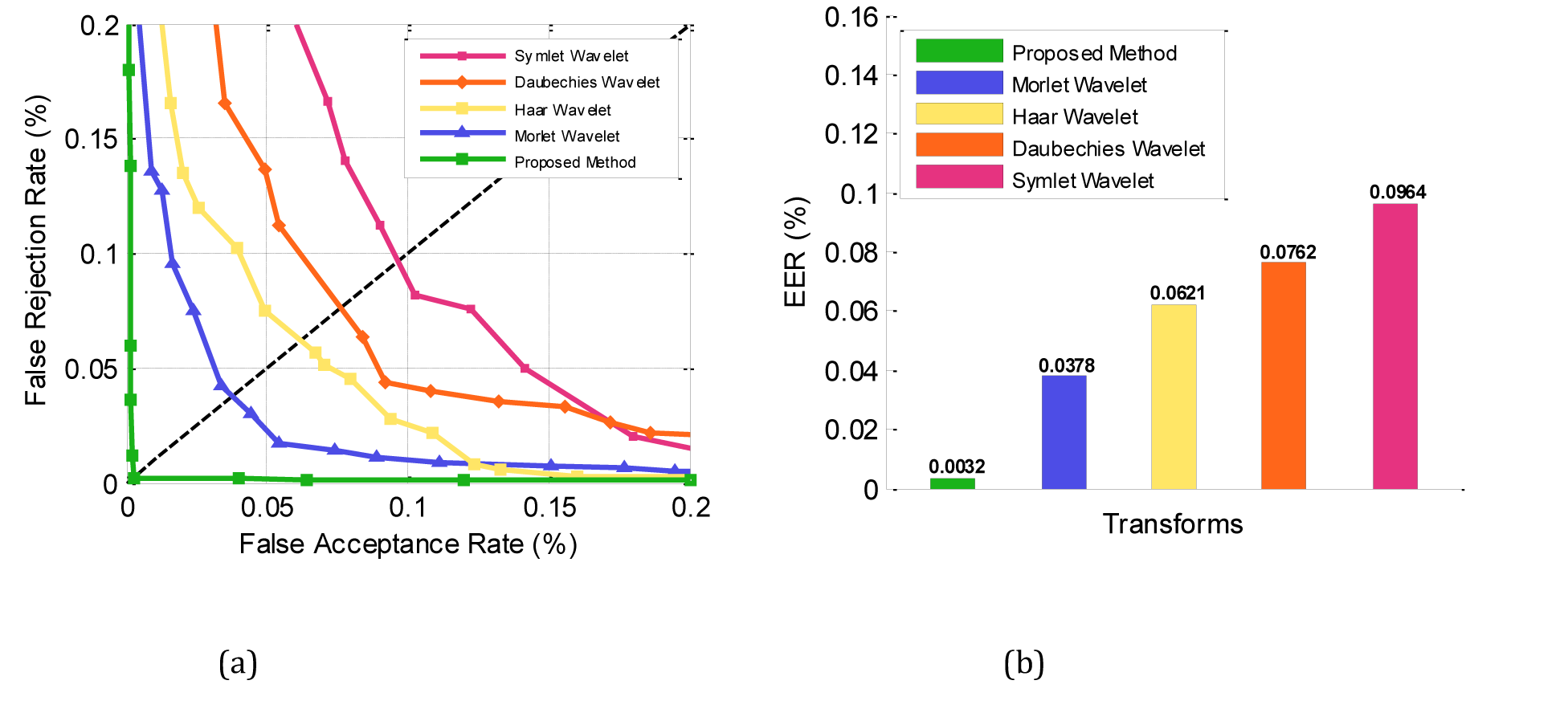
Figure 20 Comparison of ROC curves of some wavelets and contourlet transform. (a) Main comparison plot, (b) EER of each transforms.

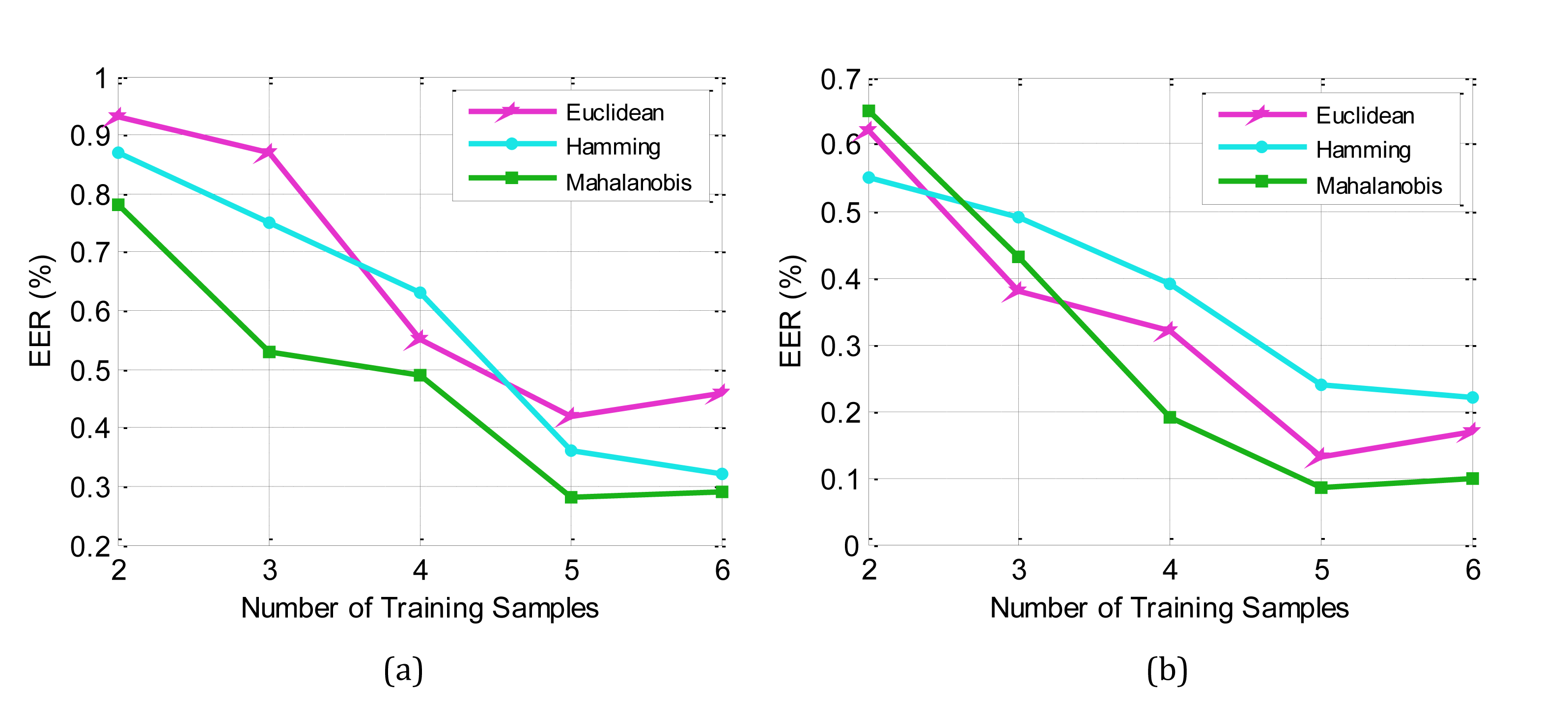
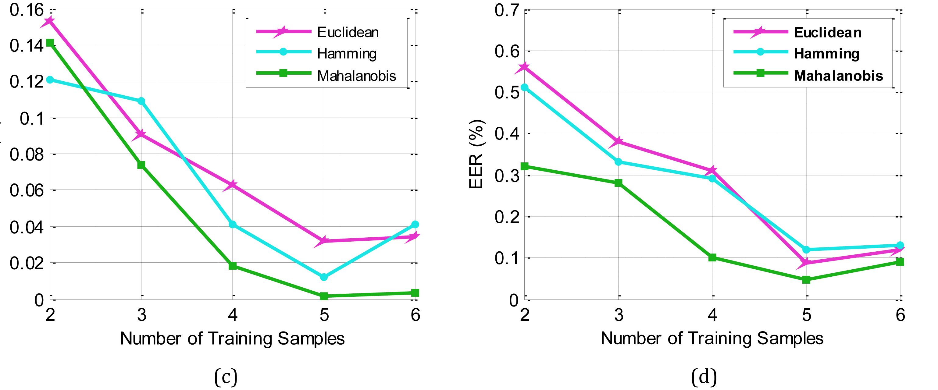
Figure 21 Comparing of matching methods at various decomposition levels: (a) 2nd level, (b) 3rd level, (c) 4th level, (d) 5th level.

Automated-based person identification is an integral element to bolster the security level, particularly in highly sensitive domains. Human retinal information gives a dependable source to biometric-based framework and is almost difficult to duplicate. The relative significance achieved by retinal scanning technology lies in:

1. Accuracy. Retinal identification offers the highest achievable accuracy and in this regard surpasses other biometric modalities, such as a fingerprint.
2. Stability of biometric sample. The blood vessels on the back of the retina are on general principle assumed to be stable throughout one’s lifetime, the exception being degenerative diseases such as diabetes.
3. The very fact that the specifics of the retinal patterns are not available to the casual observer, neither are the traces of its detail remained in daily transactions, impedes its recreation or replication. As a result, attempting to recreate or submit counterfeit retina would prove to be rather insurmountable and time-consuming, causing it to be fraud-resistant.

In this paper, we presented an automated system for person identification based on the human retina. We used a three section algorithm in this paper consisting of preprocessing, proposed methodology and feature matching. In the first step, in order to enhance performance of biometric identification system, we introduced rotation compensation and a scale invariant method based on Radial Tchebichef Moments and, further by localization of the optic disc, identified the retinal region of interest (ROI) to create the rotation invariant template from each retinal sample. The second steps involved introducing a multi-resolution analysis method based on contourlet transform. Following this, applying the proposed method, several features were extracted. In the third step, Matching function that depends on Mahalanobis distance plays out a calculation to get an arrangement and earn an arrangement of similarity scores between the present biometric example and N saved biometric templates (1: N matching).

In addition, we employed a special kind of distance to determine the similarity between the biometric patterns. Although Mahalanobis distance imposes higher computational complexity than Euclidian distance, it proves superior for typical pattern recognition applications like biometric identification; it is due mainly to its prominent features: scale invariance and features correlation exploiting. Our experimental results which are shown in Section 7, exhibit the adequacy of the proposed approach. 

Furthermore, it is possible to construct a multimodal identification by combining this technique with other biometric modalities in future works so that a new biometric identification system with greater efficiency can be achieved.

Correspondence author: Morteza Modarresi Asem. Both two authors contributed equally to the preparation of the paper, read and approved the final manuscript.

Not applicable.

The authors declare that they have no competing interests.

1. Jain AK, Ross A, Prabhakar S. An Introduction to Biometric Recognition”. IEEE Transactions on Circuits and Systems for Video Technology. 2004;14(1):4‒20.
2. Prabhakar S, Pankanti S, Jain AK. Biometric recognition: Security and privacy concerns. IEEE Security and Privacy. 2003;99(2):33‒42.
3. Simon C, Goldstein. A New Scientific Method of Identification. New York State Journal of Medicine. 1935;35(18).
4. Tower. The Fundus Oculi in Monozygotic Twins: Report of Six Pairs of Identical Twins. Archives of Ophthalmology Journal. 1955;54:225‒239.
5. Duncan D-Y Po, Minh N Do. Directional Multiscale Modeling of Images using the Contourlet Transform”. IEEE Transaction on Image Processing. 2008;15(6):1610‒1620.
6. Freeman W, Adelson E. The design and use of steerable filters. IEEE Trans Pattern Anal Machine Intell. 1991;13(9):891‒906.
7. Lee T. Image representation using 2D Gabor wavelets. IEEE Trans Pattern Anal Machine Intell. 2008;18(10): 959-971.
8. Donoho D. Wedgelets: Nearly mini-max estimation of edges. Ann Statist . 1999;27(3): 859‒897.
9. Watson B. The cortex transform: Rapid computation of simulated neural images. Computer Vision, Graphics and Image Processing Journal. 1987;39(3):311‒327.
10. Donoho D, Huo X. Beamlets and multiscale image analysis. In: Multi scale & Multi resolution Methods. Springer Lecture Notes in Computer Science Engineering Journal. 2002;20:1‒48.
11. Mallat S, Peyré G. A review of bandlet methods for geometrical image representation. Numerical Algorithms. 2007;44(3):205‒234.
12. Do M, Vetterli M. The contourlet transform: An efficient directional multi resolution image representation. IEEE Trans Image Processing. 2005;14(12):2091‒2106.
13. Labate D, Lim WQ, Kutyniok G, et al. Sparse multidimensional representation using shearlets. In Proc SPIE Wavelets XI San Diego, CA, USA. 2005;p-9.
14. Demanet L, Ying L. Wave atoms and sparsity of oscillatory patterns. Appl Comput Harmon Anal. 2007;23:1‒27.
15. Willett R, Nowak K. Platelets: A multiscale approach for recovering edges and surfaces in photon-limited medical imaging. IEEE Trans Med Imaging. 2003;22(3): 332‒350.
16. Lu Y, Do MN. Multidimensional directional filter banks and surfacelets. IEEE Trans Image Processing. 2007;16(4): 918‒931.
17. Adam Hoover, Valentina Kouznetsova, Michael Goldbaum. Locating Blood Vessels in Retinal Images by Piecewise Threshold Probing of a Matched Filter Response. IEEE Transactions on Medical Imaging. 2000;19(3):203‒210.
18. Staal J, Abràmoff M, Niemeijer M, et al. Ridge-Based Vessel Segmentation in Color Images of the Retina. IEEE Transactions on Medical Imaging. 2004;23(4):501‒509.
19. Ortega M, Marino C, Penedo MG, et al. Biometric authentication using digital retinal images. In Proceedings of the 5th WSEAS International Conference on Applied Computer Science (ACOS ’06), China. 2006;p.1‒6.
20. Tabatabaee H, Milani Fard A, Jafariani H. A Novel Human Identifier System Using Retina Image and Fuzzy Clustering Approach. In Proceedings of the 2nd IEEE International Conference on Information and Communication Technologies. 2006.
21. Ali Zahedi, Hamed Sadjedi, Alireza Behrad. A New Retinal Image Processing Method For Human Identification Using Radon Transform. IEEE, Iran. 2010.
22. Hichem Betaouaf, Abdelhafid Bessaid. A Biometric Identification Algorithm Based On Retinal Blood Vessels Segmentation Using Watershed Transformation. 8th International Workshop on Systems, Signal Processing and their Applications (WoSSPA), Algeria. (2013).
23. Seyed Mehdi Lajevardi, Arathi Arakala, Stephen A Davis, et al. Retina Verification System Based on Biometric Graph Matching, IEEE Transaction on Image Processing. 2013;22(9):3625‒3635.
24. Oinonen H, Forsvik, P Ruusuvuori H, et al. Identity Verification Based on Vessel Matching from Fundus Images. In 17th International Conference on Image Processing, Hong Kong. 2010.
25. Farzin H, Abrishami Moghaddam H, Moin MS. A novel retinal identification system. EURASIP Signal Process Journal. 2008: 280635.
26. M Ortega, MG Penedo, J Rouco, et al. Retinal Verification Using a Feature Points-Based Biometric Pattern. EURASIP Journal on Advances in Signal Processing. 2009.
27. Majid Shahnazi, Maryam Pahlevanzadeh, Mansour Vafadoost. Wavelet Based Retinal Recognition. International Symposium Signal Processing and its Applications of IEEE. 2007.
28. Joddat Fatima, Adeel M Syed, M Usman Akram. A Secure Personal Identification System Based on Human Retina. IEEE Symposium on Industrial Electronics & Applications, IEEE, Malaysia. 2013.
29.  Xianjing Meng, Yilong Yin, Gongping Yang, et al. Retinal Identification Based on an Improved Circular Gabor Filter and Scale Invariant Feature Transform. Sensors (Basel). 2013;13(7):9248‒9966.
30. Joewono Widjaja. Noise-robust low-contrast retinal recognition using compression- based joint wavelet transform correlator. Optics & Laser Technology Journal. 2015;74: 97‒102.
31. Zahra Waheed, M Usman Akram, Amna Waheed, et al. Person identification using vascular and non-vascular retinal features. Computers and Electrical Engineering. 2016;53:359‒371.
32. KG Goh, W Hsu, ML Lee, et al. An automatic diabetic retinal image screening system. In Medical Data Mining and Knowledge Discovery, Springer, Germany. 2000.
33. Michael D Abràmoff, Mona K Garvin, Milan Sonka. Retinal Imaging and Image Analysis. IEEE Rev Biomed Eng. 2010;3:169‒208.
34. R Mukundan, SH Ong, PA Lee. Image Analysis by Tchebichef Moments. IEEE Transactions on Image Processing. 2001;10(9).
35. R Mukundan. Radial Tchebichef invariants for pattern recognition. Proc of IEEE Tencon Conference-TENCON, Australia. 2005.
36. H Hanaizumi, S Fujimura. An automated method for registration of satellite remote sensing images. Proceedings of the International Geoscience and Remote Sensing Symposium IGARSS’93, Tokyo, Japan. 1993.
37. MN Do, M Vetterli. Contourlets in Beyond Wavelets. In: GV Welland (Eds.), Academic Press, New York, USA. 2003.
38. Minh N Do, Martin Vetterli. The contourlet transform: an efficient directional multiresolution image representation. IEEE Trans. Image Proc. 2008;14(12):2091‒2106.
39. Candes E, L Demanet, D Donoho, et al. Fast Discrete Curvelet Transforms. Multiscale Model Simul. 2006;5(3): 861‒899.
40. Burt PJ, EH Adelson. The Laplacian Pyramid as a compact image code. IEEE Trans on Commun. 1983;31(4):532‒540.
41. Song H, Yu S, Song L, et al. Contourlet Image Coding Based on Adjusted SPIHT. Springer-Verlag Berlin Heidelberg Journal. 2005.
42. Liu Z. Minimum distance texture classification of SAR images in contourlet domain. In: Proceedings of the International Conference on Computer Science and Software Engineering, India. 2008.
43. Katsigiannis S, Keramidas EG, Maroulis D. Contourlet transform for texture representation of ultrasound thyroid images. IFIP Advances in Information and Communication Technology Journal. 2010.
44. Jain A, Nandakumar K, Ross A. Score Normalization in multimodal biometric systems. Pattern Recognition. 2005;38(12): 2270‒2285.
45. Supriya Kapoor, Shruti Khanna, Rahul Bhatia. Facial gesture recognition using correlation and Mahalanobis distance. International Journal of Computer Science and Information Security. 2010;7(2).
46. Chul-Hyun Park, Joon-Jae Lee, Mark JT Smith, et al. Directional Filter Bank-Based Fingerprint Feature Extraction and Matching. IEEE Trans. Circuits and Systems for Video Technology. 2004;14(1):74‒85.
47. Köse CA. Personal identification system using retinal vasculature in retinal fundus images. Expert Systems with Applications. 2011;38(11):13670‒13681.
48. Sukumaran S, Punithavalli M. Retina recognition based on fractal dimension. IJCSNS Int J Comput Sci and Netw Secur. 2009;9(10).
49. Barkhoda W, Tab FA, Amiri MD. A Novel Rotation Invariant Retina Identification Based on the Sketch of Vessels Using Angular Partitioning, In Proceedings of 4th International Symposium Advances in Artificial Intelligence and Applications, Poland. 2009;p.3‒6.
50. Amin Dehghani, Zeinab Ghassabi, Hamid Abrishami Moghddam, et al. Human recognition based on retinal images and using new similarity function. EURASIP Journal on Image and Video Processing. 2013.
51. ZW Xu, XX Guo, XY Hu, et al. The blood vessel recognition of ocular fundus. In Proceedings of the 4th International Conference on Machine Learning and Cybernetics Guangzhou. 20 05.