Sample size determination continues to be an important research area of statistics. Perhaps nowhere is this truer than pharmaceutical statistics, where cost and time constraints have made finding the appropriate sample size before conducting a study of the utmost importance. The problem is quite simple: too small a sample can lead to under-powered studies, while too large a sample size wastes precious resources. In this article we consider the sample size determination problem as it pertains to the two-sample testing of Poisson rates from a Bayesian perspective subject to operating characteristics constraints.
There are several advantages to the Bayesian perspective when trying to determine a study's requisite sample size, a topic that is expounded in Adcock.1S Their construction does not depend on asymptotic approximations or bounds. Classical solutions to the sample size determination problem typically hinge on asymptotic arguments that require the researcher to specify one parameter value (perhaps vector valued) as representative for the entire parameter space, a process that is typically done using bounding arguments. This, for example, is what is done when determining the requisite sample size for a confidence interval of a fixed level and given length. The resulting sample sizes are consequently conservative. On the other hand, the Bayesian approach provides the statistician with the ability to model his indecision about the parameter through expert knowledge or previous studies. As noted by Bayarri and Berger,2 this can allow the Bayesian approach to have better operating characteristics, such as a smaller required sample sizes or better Type I and II error rates.
Various Bayesian sample size determination methods have been studied for binomial and Poisson data. Stamey et al.3considered one and two sample Poisson rates from the perspective of interval based criteria such as coverage and width. Hand et al.4 extend those ideas by considering both interval-based and test-based criteria, albeit without considering power. Katsis and Toman5 used more decision theoretic criteria for the two sample binomial case, but only to the extent of controlling the posterior risk with a pre specified bound. Zhao et al.6 extend those ideas by using computational methods to consider expected Bayesian power of the test. In this article, we extend these results to the Poisson data model. We also consider the problem the subject to Type I and Type II constraints. This is thus an important extension of,6 because it
- Extends the ideas to the Poisson case
- Enables the incorporation of operating characteristics.
A subtle difference between the classical and Bayesian methods of sample size determination merits discussion before proceeding. One of the novel contributions of this article is an algorithmic solution to the sample size determination problem subject to operating characteristics constraints for Poisson data. However, since the entire problem is treated in a Bayesian context, the concept of Type I and Type II error rates is understood in an average, or expected, sense; see.7 For example, the ``power of a test'' retains the interpretation of the probability the decision rule rejects when the null hypothesis when it is false; but rather than being a function defined over the alternative space, here it is averaged over that space and weighted by the prior distribution specified on the alternative hypothesis. To make the distinction more clear, we refer to this as the expected Bayesian power (EBP), as is done in;8 alternatively, it may be referred to as the probability of a successful test. These ideas, though apparently not considered in the literature previously, can also apply to the concept of the significance level of a test. While frequentist methods typically report one value for significance level, what they are really doing (in non point null hypotheses) is taking the largest possible significance level; thus, taking an expectation of a significance level curve could be done as well. Consequently, in this article we also consider the expected Bayesian significance level (EBSL), defined as the expected value of the test under the prior distribution given on the null space. In both cases, any particular instance of the actual Type I and Type II error rates can be greater than or less than nominal.
This article proceeds as follows. In Section 2 we introduce the theoretical formulation of the sample size determination problem for two Poisson variates including consideration of operating characteristics. In Section 3, we present an algorithmic solution to the sample size determination problem posed in Section 4. Section 5 contains an application of the method in the area of pharmaceutical statistics. We then conclude with a discussion.
Problem specification and the bayes rule
We now follow the general framework of6 in the development of this problem, adapting the binomial case to fit the Poisson data model. Suppose
and
, independently, where
and
represent the rate parameters of interest and t represents a common sample (or “opportunity”) size. Together, we write these
with observations
. The sample size determination problem is to calculate the necessary sample size required to test the hypotheses
vs
using a given decision rule; here we use the Bayes rule. Denoting the parameter pair
, the associated null and alternative spaces are therefore
which we identify with
with elements generically denoted
, and
.
As this problem is being considered from the Bayesian perspective, we place prior probabilities of
and
on
and
, respectively. Conditional on the null being true, we represent the expert opinion regarding
as
, defined over the set
. Alternatively, conditionally on
being true, we represent the belief concerning
with a joint prior
with support
. Marginalizing over the hypotheses, we have the unconditional prior
Where
and
are the indicator function of
and
, respectively.
In practice, the prior distributions on
,
, and
summarize expert opinion concerning the parameters in each of the two scenarios
and
. This information can be obtained in a number of ways including past data, prior elicitation of expert opinion (see especially9), or based on uninformative criteria. For simplicity, we consider conjugate priors for all three
’s, so that under
,
, and under
,
independently. This assumption is not very restrictive and allows us to specify parameters of prior distribution sin stead of distributions themselves.
We now derive the optimal Bayes (decision) rule in deciding between the hypotheses presented in (1). In solving the related problem between two binomial proportions,6 use the classical decision theoretic setup using the 0-1 loss function.10 Here we use the more general unequal loss function
Where
is the decision rule with a = 0 representing selection of
and a = 1 selection of
. Thus, c1 represents the loss associated with a Type I error, and c2 that of a Type II error.
The Bayes action is simply the one that minimizes posterior expected loss.11 Since the posterior expected loss associated with an action
is
Setting
we can express the optimal decision rule,
, as
The rejection region,
, is therefore
The optimal rule in (2) can be nicely represented in terms of the Bayes factor. The Bayes factor is defined as the ratio of the posterior odds of to the prior odds of
, so that a large Bayes factor is evidence for rejecting the null hypothesis.12 Specifically, the Bayes factor is defined
This ratio is useful in Bayesian inference because it is often interpreted as partially eliminating the influence of the prior on the posterior, instead emphasizing the role of the data. Moreover, the decision rule is a function of a Bayes factor:
=
This is particularly useful because it allows for the interpretation of the Bayes factor B as the test statistic for the decision rule in (2); this is the condition in (4).
We now derive closed-form expression for the posterior probabilities of the null and alternative hypotheses. Using Bayes’ theorem, we have
and
.
Consequently, the posterior probabilities have closed-form expressions if the likelihoods do. Computing these, we have
and
Note that the probability of the data under the null hypothesis is the product of two independent negative binomial likelihoods.
Combining (3) with (5) and (6) allows us to represent W in terms of the null and alternative likelihoods as follows:
Consequently, (7) and (8) give explicit conditions for the rejection of the optimal decision rule:
Note that the left side of (9) is our test statistic and Bayes factor, B, so that (9) is an explicit formulation of the condition presented in (4).
Sample Size Determination for the Bayes Rule
The explicit description of the decision rule in (9) allows us to compute all sorts of quantities of interest. For given prior parameters
,
, α, β,
, ,
, and
and loss penalties
and
(or simply c), the Expected Bayesian Power (EBP)
is defined
and the Expected Bayesian Significance Level (EBSL)
is
Note three things. First the inclusion of the t subscripts highlights the fact that these quantities depend on t. Second, both
and
marginalize over the corresponding alternative and null spaces
and
, respectively, this is the sense in which the power and significance level are expectations. Third, the constant c (or c1 and c2) is represented in the expressions through Wt, which is itself dependent on t.
In their articles,5,12 demonstrate that as the sample size tends to infinity, the Bayes factor converges to either 0 or 1. As a consequence, in the current context as the sample size t tends to infinity the Bayes factor
converges to either 0 or 1, so that12 implies that
and
. Thus, for any pre-specified power
and significance level
, there exists a t such that for all
,
and
. We define
to be the in fimum of this collection of lower bounds, i.e.
is said to be the optimal sample size for
and
, and computing
is called the sample size determination problem. If only a power is specified, or if only a significance level is specified, the other quantity is left off of the subscript and out of the definition. We often write simply
for
.
Were (10) and (11) monotonic and continuous in
t, the sample size determination problem would be quite straightforward. Simply run a numerical root-finder (e.g. Newton's method) on
and
take the larger
t. Unfortunately, however, as a function of
t both the power and significance level are discontinuous functions that are not monotonic. As a consequence, it is possible, for example, for there to be two such sample sizes
t1and
t2 with
such that
and yet
. This is a consequence of the dependence of
Wt on
t: as
t grows, the rejection region changes, and these changes result in discrete jumps in the rejection region.
Practically speaking, in our experience the appearance of these jumps is monotonically decreasing in magnitude and dissipate quite quickly in t so that, while there are jumps, they become relatively minor even for quite small t. Thus, while out-of-the-box numerical routines are insufficient for the task, a straight-forward heuristic algorithm suffices to certify
to a reasonable level of accuracy.
Initialize
with a value small enough to satisfy
and
, typically a value like .1 will suffice. Then, double t until both conditions are met. Once both conditions are met, decrement t by 1 until the conditions are no longer satisfied; then decrement by .1, and so on to achieve the desired precision. Alternatively, one may move in a binary search manner; this method is faster but loses the certificate of the solution up to the highest evaluated point. By contrast, the first heuristic certifies that the sample size achieved is optimal up to the largest t observed, which is of the form
.
One computational detail is relevant for implementing this procedure. By definition, since
and
are Poisson variates, their sample spaces are infinitely large, and thus computing
and
is not numerically possible - one cannot check every
to determine whether or not it is included in Wt. There is, however, a very reasonable work-around for this problem using prior predictive distributions. Under H1, the prior predictive distributions on
and
are both negative binomial. Specifically,
and
While one cannot enumerate the entire sample space of , one can be confident they have a satisfactory approximation by computing small (e.g. .00001) and large (e.g. .99999) quintiles of these distributions and then simply taking every combination of the ranges from low to high. This is the approach we take to computing the sums listed in (10) and (11) above.
An Example from Cancer Therapeutics
- An example of the proposed methodology is readily available from the field of cancer therapeutics. Suppose (1) Drug A is an industry standard therapy for a certain type of cancer that is known to have the common side effect of mild seizures every hour of infusion
- (2) Drug B is a novel compound believed to have the same side effect but at a lessened rate
- (3) The goal is to design a design a clinical trial that compares the two using the minimum resources required to meet 5% significance level (EBSL) and 80% power (EBP). Moreover, suppose that the losses associated with Type I and Type II errors have a ratio of 1:1.
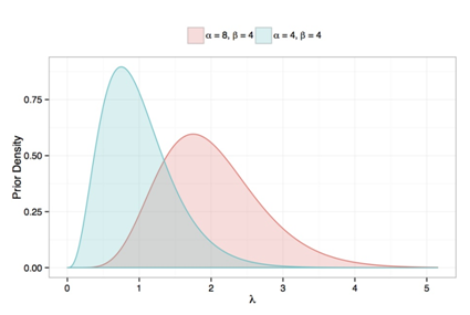
From past studies, it is known that the uncertainty in the rate of seizures with Drug A (per hour) is well-represented by a Gamma (4, 4) distribution so that
. Drug B, by contrast, is believed to be a bit worse, with perhaps a rate that is double that of Drug A with experts 90% sure the value is less than about 3. This translates into roughly
. Figure 1 shows both of these priors graphically.

Figure 1 Prior structures used in Poisson sample size determination example.
Assuming that the rates are the same, the past indicators of Drug A supersede the lack of evidence for Drug B, so that under the null hypothesis
is most appropriate. Assuming that the null and alternative hypotheses are given the same belief (50%), the rejection rule from (9) is therefore
(12)
(13)
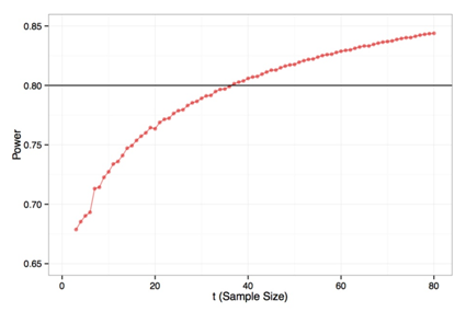
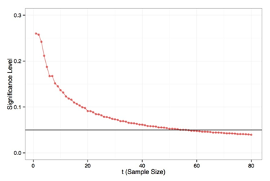
To design a test with 80% power and at the 5% significance level, we need but to run the algorithm described in Section 3. To illustrate the scenario, we plot the significance level and power for every t from 1 to 80; these are included in Figures 2 and Figure 3, respectively. Note how quickly (in t) the functions become smooth, nullifying any concern about jumps. The 80% level is achieved at t = 37, with a power of 80.1%, and the 5% significance level is achieved at t = 57, where the significance level is 4.9%. Thus, to achieve both, we select the higher sample size, t = 57.


We can also verify these results via simulation by generating one million random values of
and
from the priors given above. To validate the significance level result, we simply (1) sample from the prior, (2) generate two Poisson observations with mean equal to the sample in (1) times 57, and (3) determine whether the test rejects (1) or not (0). Averaging the million test results, the value is confirmed to Monte Carlo error (code available upon request). To validate the power result, we (1) sample one number from a Gamma(4, 4)and one number from a Gamma(8, 4), (2) sample two Poisson observations from distributions with mean 37 times the two variates generated in (1), and (3) determine whether the test rejects or not. Averaging the million results validates the theoretical result.


