The phenotype of an individual depends upon both the genetic make-up and environmental influences. Genotype × environment interaction is considered as an important source of discrepancy in any crop, and different methods have been used to distinguish genotypes for their behavior in different environmental conditions. These constitute univariate parametric, such as environmental variance, regression slope, and deviation from regression, to multivariate methods. In this review, we summarize the priorities and limitations of different parametric stability statistics, and also their correlations which might help agronomists and crop breeders to choose the proper methods for their analysis.

Keywords: genotype by environment interaction, performance, stability

Yield stability has always been considered as an important topic in plant breeding but will be more concern by the continued variation in climatic condition. The phenotype of an individual is a mixture of both genotype (G) and environment (E). As a consequence of G × E interaction, crop varieties may not show uniform performance across different environments. The term genotype refers to the genetic makeup of an organism while environment refers to biophysical factors that have an effect on the growth and development of a genotype.¹ The G × E study is especially important in countries with various agro-ecologies. Significant G × E interaction is a consequence of variations in the extent of differences among genotypes in diverse environments (called as a qualitative or rank changes) or variations in the comparative ranking of the genotypes (called as a quantitative or absolute differences between genotypes)^2–4

Stability definition
All performance stability, phenotypic stability, and adaptation terms are usually used in total various meanings and different senses and explanations are introduced over the years.^5,6 In a static mean of stability defined by Becker and Leon,⁶ a stable genotype is the one possessing a constant performance irrespective of any changes in environmental conditions. According to Peterson et al.,⁷ the optimal genotype stability definition and response for quality parameters varies relatively from that conventionally used to characterize yield stability. For breeders, stability of quality properties is important from the points of changing genotypes ranks’ throughout environments and influences selection efficiency. For end-users, such as millers and bakers, stability in quality properties of genotypes is more important, irrespective of genotypes rank changes. However, as pointed out by Grausgruber et al.,⁸ the quality of a genotype often behaves similar to other quantitative characters to desirable and undesirable environmental conditions. As a result, a genotype is regarded stable if it has a low contribution to the G × E interaction.

Basic concepts

In the final stage of plant breeding, the new varieties are grown under different seasons of the year, environments, climatic and soil conditions.^6,9 Environments and seasons, in the role of different conditions, are specified to be a single factor for environmental conditions. The most commonly used designs in these experiments are randomized complete blocks and incomplete block designs. For the latter, owing to the large number of genotypes, lattice designs are usually used. In all experiments, plant breeders usually focus on modeling the genotype means estimated in the jth environment. Therefore, one may consider the linear model: 

$Y_{ij}=\mu +g_i+e_j+g{e}_{ij}+e_{ij}$ (1)

where: $Y_{ij}$  is the observed mean of the $i^{th}$  genotype at the $j^{th}$ environment, for $i=1,2,\mathrm{...},n$ , and $j=1,2,\mathrm{...},n;\mu$ is the overall mean of the $i^{th}$  genotype; $g_i$  is the effect of the $i^{th}$  genotype, $e_j$  represents the effect of the $j^{th}$ environment, $g{e}_{ij}$  is the effect of interaction between $i^{th}$  genotype and $j^{th}$ environment, $e_{ij}$  is the mean error related to the observed $Y_{ij}$

The $G\times E$  interaction (term $g{e}_{ij}$ in equation 1) can be explained as the differential yield response of a genotype to environments. As a direct consequence of $G\times E$  interaction, the approximate performances of two genotypes vary with the environment stimuli. As a result, one of the most significant goals of the phenotype stability analysis is to distinguish the genotypes whose phenotypic performance remains constant while the environmental conditions change. In the presence of $G\times E$  interaction, these analyses make sense.¹⁰ Radiation, water, and nutrients availability are among the factors which strongly influence crop growth and yield¹¹ therefore, the components of phenotypic variance may often rank as follows:^12–20
${\sigma }^2{}_E > G \times E > {\sigma }^2{}_G$
In contrast to the above ranking, in a study by Puttha et al.,²¹ the genotype contributed to a large proportion of variation in inulin content and fresh tuber yield, whilst and environment had a smaller contribution to discrepancies. The difference in contrast is feasibly largely because of materials used and environments’ conditions. In other studies, it was observed that the G × sowing seasons (SS) interaction was less important than the $G\times E$ year interaction.²² These results show that the evaluation of genotypes based on several environments and years is more important than the evaluation for the two seasons.

Illustration of $G\times E$effect
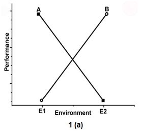
To show the environmental effect, the 2 genotypes called A and B, are tested in two environments (E1 and E2) in Figure 1.  Figure 1a indicates the presence of an interaction effect in which genotype A is superior to genotype B in E1 but has the lowest mean in E2.  Figure 1 b shows the absence of $G\times E$interaction.

Figure 1a Indicates the presence of an interaction effect in which genotype A is superior to genotype B in E1 but has the lowest mean in E2.

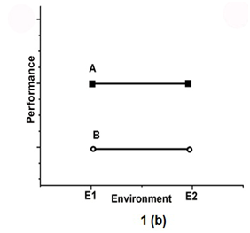
Figure 1b Shows the absence of interaction.

Methods for estimating phenotypic stability
The economic significance of stability for the cultivation of a genotype was first identified by Roemer [1917, cited in 8] who used the variance across environments as a parameter for yield stability. This stability parameter follows a biological/static sense implicating that a stable genotype is recognized as the one having small variance across the tested environments.⁶ Therefore, to estimate the static phenotype stability of the $i^{th}$  genotype, the following equation can be used:
$S^2{}_{xi}$  = $\frac{{\displaystyle \sum _{}^{}{(X_{ij}-{\overline{X}}_{i.})}^2}}{E-1}$                              (2)
where $X_{ij}$  is the performance of the $i^{th}$  genotype in the $j^{th}$  environment, $X_i{}_{.}$ is the mean performance of the $i^{th}$ genotype and $E$  is the number of environments.

If the sample estimate is not significantly different from zero, a genotype is then recognized to be stable which means that environmental changes will not influence the genotype performance. However, this type is rarely a favored feature of crop landraces, inasmuch as genotypes with high phenotypic stability obtained through the environmental change have low yield. As a result, this method does not desired by plant breeders to evaluate the phenotypic stability of the genotype performance, or other related random variables. Although, it is helpful to evaluate the phenotypic stability of the traits that should retain their levels such as stress characters like winter hardiness, qualitative traits, or disease resistance.²³ In contrast, if a genotype response to environmental changes has no deviation from the general response of all genotypes in the trial, it is called as dynamic or agronomic stability. The dynamic concept of stability is useful for quantitative traits such as yield.²³

Using the dynamic concept of stability, Wricke’s^25,25 model is the simplest method to evaluate the stability. Wricke^25,25 suggested the ecovalence (W2i) concept as the ratio of the interaction sum of squares contributed by each genotype to the $G\times E$ interaction sum of squares. In other words, the ecovalence of the $i^{th}$  genotype is its interaction with the environments, squared and summed across environments, and expressed as
$W_i^2={\displaystyle \sum {\left(X_{ij}-{\overline{X}}_{i.}-{\overline{X}}_{.j}+\overline{X}\mathrm{..}\right)}^2}$                   (3)
Where $X_{ij}$  is the mean performance of the $i^{th}$  genotype in the $j^{th}$  environment and $X_{i.}$ and $X{.}_j$  are the genotype and environment mean deviations, respectively, and $X_{\mathrm{..}}$ is the overall mean.  For this reason, genotypes with a low $W^2{}_i$  value have smaller deviations from the mean across environments and are therefore more stable.  Based on Becker and Leon,⁶ a genotype with $W^2{}_i=0$ is considered stable.

Shukla²⁶ proposed the variance component of each genotype across environments as another relevant measure of phenotypic stability. It measures stability rather than performance. According to Shukla²⁶ stability variance $({\sigma }^2{}_i),G\times E$  sum of squares is partitioned into components, one corresponding to each genotype and estimated as
${\sigma }^2{}_i=\frac{1}{(G-1)(G-2)(E-1)}\left[G(G-1){\displaystyle {\sum }_j}{(X_{ij}-{\overline{X}}_{i.}-{\overline{X}}_{.j}+{\overline{X}}_{\mathrm{..}})}^2-{\displaystyle {\sum }_i}{\displaystyle {\sum }_j}{(X_{ij}-{\overline{X}}_{i.}-{\overline{X}}_{.j}+{\overline{X}}_{\mathrm{..}})}^2\right]\mathrm{...}$    (4)
Where G is number of genotypes, E is number of environments, $X_{ij}$  is the mean yield of the $i^{th}$  genotype in the $j^{th}$  environment, $X_i.$ is the mean of the $i^{th}$  genotypein all environments, $X{.}_j$  is the mean of all genotypes in $j^{th}$ environments and $X\mathrm{..}$ is the overall mean.

If the stability variance of a genotype was equal to the environmental variance$({\sigma }^2{}_i=0)$ , then genotype is identified as stable. A slightly large value of ${\sigma }^2{}_i$  will therefore illustrate more instability of the $i^{th}$ genotype. Significant ${\sigma }^2{}_i$  value’s also shows that a genotype’s performance throughout the environments was unstable. Genotypes with a non significant or negative ${\sigma }^2{}_i$  would be regarded stable throughout the environments.²⁶ Since σ2i is the difference between two sums of squares, negative ${\sigma }^2{}_i$  may sometimes occur which can be considered as equal to zero in such conditions.²⁶ It is also important to note that ${\sigma }^2{}_i$ cannot be computed from unbalanced data.²⁷

The level of correlation among different stability parameters represents whether one or more parameters should be used for cultivar performance prediction, and also gives breeder the right to choose the best stability parameter(s) to fit the sense of stability.²⁸  Shukla²⁶ stability variance is a linear combination of deviation mean squares, in other words the Wricke^24,25 ecovalance. Significant positive correlation between $W^2{}_i$  and ${\sigma }^2{}_i$ was found in different studies (Table 1) which indicates that $W^2{}_i$ and${\sigma }^2{}_i$ are equivalent in ranking genotypes for stability [29-33]. As a result, it is adequate and acceptable to use one of the two statistics solely.³⁴ However, in a study by Kang et al.,³⁵ Shukla²⁶ method was preferred to Wricke^24,25  for estimating the yield stability of sugar cane cultivars. Contrary to the results of previous studies (Table 1), Akcura et al.³⁶ reported a significant negative association (-0.88, P < 0.05) between ${\sigma }^2{}_i$  and $W^2{}_i$ .

The main type of stability analysis called joint regression analysis or joint linear regression (JLR) was termed by Freeman.³⁷ It helps to estimate whether the genotypes have characteristic in a linear responses to environmental changes. The interaction sum of squares is partitioned into two parts: one describes the heterogeneity of linear regression coefficient $\left(b_i\right)$  whereas the second represents a deviation$\left(d_{ij}\right)$ :
${(G\times E)}_{ij}=b_i{E}_j+d_{ij}$ (5)
and therefore
$Y_{ij}=\mu +G_i+E_j+\left(b_i{E}_j+d_{ij}\right)+e_{ij}$ (6)
Where $E_j$  is the environmental index, $b_i$  is the regression coefficient that measures the response of the genotype of varying environments, $d_{ij}$  stands for the deviation from regression of the $i^{th}$  genotype at the $j^{th}$  environment, and the remaining stands as specified in equation 1. The joint regression analysis approach was first introduced by Yates and Cochran³⁸ and was later modified by Finlay and Wilkinson³⁹ and Eberhart & Russell⁴⁰ which is a widely used method nowadays.

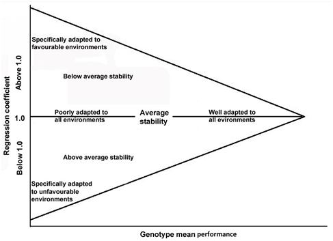
Figure 2 Genotype regression coefficients plotted against genotype performance, adapted from Finlay and Wilkinson.³⁹

The regression coefficient was introduced by Finlay and Wilkinson³⁹ as the regression of the mean of $i^{th}$ genotype in $j^{th}$ environment on the mean performance of all genotypes in that environment and is expressed as
$b_i=1+\frac{{\displaystyle {\sum }_i}\left(X_{ij}-{\overline{X}}_{i.}-{\overline{X}}_{.j}+\overline{X}\mathrm{..}\right)\left({\overline{X}}_{.j}-\overline{X}\mathrm{..}\right)}{{\displaystyle {\sum }_j{\left({\overline{X}}_{.j}-\overline{X}\mathrm{..}\right)}^2}}$   (7)
where $X_{ij}$  is the performance of the $i^{th}$ genotype in the $j^{th}$ environment, $X_{i.}$ Is the mean performance of the $i^{th}$ genotype, and $X_{.j}$  is the mean performance of the $j^{th}$ environment, $X\mathrm{..}$ is the overall mean and E is the number of environments. The regression coefficient $\left(b_i\right)$ mainly indicates the adaptation of a genotype to several environments and also describes the linear response between environments. However, it does not reflect stability, crop performance, or stability extension.^40,41

As it could be seen in Figure 2, a genotype which has a regression line above that for overall mean performance is regarded to have high performance stability and is able to adapt to all environments. As the productivity of the environment improves, the performance of such genotype would increase. A genotype is considered to have adaptation to a specific environment if its regression line crosses that for overall mean performance. A genotype is regarded to have low performance adaptability across environments if its regression line placed below that for the overall mean performance.³⁹ The slope of regression line showed a positive association with yield potential in different studies^{16,32,42–46} which means that high yielding genotypes have larger values for bi which are particularly adapted to environments with favourable growing condition. Therefore, such genotypes, when cultivated in poor environments would show less than optimal performance but when cultivated in optimal environments, they could achieve maximum performance.

Altay⁴⁷ suggested that Finlay and Wilkinson³⁹ method is a preferable method for the assessment of specific or wide adaptation of genotypes compared with Wricke^24,25 ecovalence.

Eberhart and Russell⁴⁰ suggested using the mean of squared deviations from regression $\left(S^2{}_{di}\right)$ as a measure for stability and a stable genotype is the one has a small deviation from regression mean squares (equation 8).
${{\displaystyle S}}_{di}^2=\frac{1}{E-2}\left[{\displaystyle {\sum }_i}{(X_{ij}-{\overline{X}}_{i.}-{\overline{X}}_{.j}+\overline{X}\mathrm{..})}^2-{(b_i-1)}^2{\displaystyle {\sum }_i}{({\overline{X}}_{j.}-\overline{X}\mathrm{..})}^2\right]$         (8)
where all components have their usual meanings.

According to Eberhart and Russell⁴⁰ model, genotypes are grouped based on their variance of the regression deviation (either equal or not to zero). A genotype with variance in regression deviation equal to zero is highly predictable, whilst a genotype with regression deviation more than zero has less predictable response [48]. Although, regression model is displayed to be the most useful approach for geneticists^37,48–51 but authors have found a number of statistical and biological restrictions and criticisms.

One of the drawbacks of this analysis is that the mean of all genotypes in each environment is considered as a measure of the environmental index and is used as an independent variable in the regression. According to the regression analysis assumptions, no independence can be among the variables, particularly when the number of genotypes is less than 15.^6,52 In addition, the variation in regression coefficient result is most often so small which makes it difficult to rank the genotypes for stability and adaptability. Regression analysis should be used with caution when only a few low or high performance sites are included in the analysis;^51,52 since the genotype fit may be determined greatly by its performance in a few extreme environments, it leads to the generation of misleading results.

A strong positive relationship between $S^2{{}_d}_i$  and ${\sigma }^2{}_i$  was found in studies on durum wheat, lentil, maize, and pea (Table 1) and also between $S^2{{}_d}_i$ and $W^2{}_i$  for durum wheat, lentil, maize, pea, popcorn, sorghum, and soybean cultivars (Table 1). Jowett⁵³ concluded that the Eberhart and Russell⁴⁰ method, which uses an arithmetic scale, was more explicit than the Finlay and Wilkinson procedure, which uses a logarithmic scale. Stability parameters such as $S^2{{}_d}_i$ ,$W^2{}_i$ , and ${\sigma }^2{}_i$ were found to be useful in assessing the phenotypic stability of field genotypes.^3454–57  Marjanovic-Jeromela et al.⁴⁵ found a negative correlation between $W^2{}_i$ and $S^2{{}_d}_i$ which indicates that either of these two methods could be used independently from each other without influencing accuracy of estimation.

Joint regression and QTL mapping
Two possible genetic mechanisms including the allelic sensitivity and gene regulation models are proposed for supporting stability.^58,59 In the first model and in direct response to the environment, the constitutive gene regulates itself through the activation of different alleles in various environments.

Regardless of how stability is expressed or measured, one of the most important questions for a stability parameter is whether it is genetic.⁶⁰ Two possible genetic mechanisms are proposed for underpinning stability;^58,59 the allelic sensitivity model, which suggests that the constitutive gene is regulated itself in direct response to the environment through the activation of different alleles in various environments. The gene regulation model implies that one or more regulatory loci are under the direct influence of the environment and the constitutive gene is switched on or off by the regulatory gene. Collocation of QTLs (a segment of DNA that influences a quantitative trait) illustrating $G\times E$  interactions and QTLs for stability parameters would support the allelic sensitivity model,^59,61 whilst QTLs for stability parameters detected in regions other than those for the trait would imply a regulatory model.^62,63 Joint regression analysis is widely used in quantitative genetics to analyze QTL × environment interaction.^59,64 Previous studies found that the deviation from regression is not under genetic control,^59,65 which is in contrary to the findings of Kraakman et al.⁶¹

Perkins and Jink⁶⁶ introduced a statistical analysis to measure non linear sensitivity to the environmental variations by considering the $G\times E$ interaction component of each genotype as a linear function of the additive environmental component. In this model, the deviation from the regression line of each environment is considered as a fixed effect and a genotype with ${\beta }_i=0$ and ${\sigma }^2{}_i=0$ is regarded as stable. The $b$  -values^38–40 have a mean of unity, while the $\beta$  -values^6,26 have a mean of zero.

In a study by Annicchiarico and Mariani,⁶⁷ 9 wheat lines were grown at six Italian locations for three seasons. Positive correlation between $\beta$ -values and ${\sigma }^2{}_i$ indicated lines adaptability with generally low yield stability.

Lin and Binns⁶⁸ proposed the superiority measure $(P_i)$ of the $i^{th}$  genotype as the performance difference comparison among a set of genotypes compared with a reference genotype with the maximum performance within each environment:
$P_i=\frac{\left[{\displaystyle \sum _{j=1}^n}{(X_{ij}-M_j)}^2\right]}{2E}$                          (9)
Where $X_{ij}$  is the average performance of the $i^{th}$  genotype in the $j^{th}$  environment, $E$  is the genotype with maximum performance among all genotypes in the $j^{th}$ environment, and $E$  is the number of environments.

Small $P_i$  value’s indicates less distance between the $i^{th}$ genotype and the genotype with maximum performance and the better the genotype.^69,70 This explanation of superiority is compared to the breeder’s purpose, because a superior genotype should be placed among the most productive genotypes across environments.

Although, Lin and Binns⁶⁸ method is seldom used in different studies but it does not have   restrictions of the regression model. In this method, the stability statistics are on the basis of both the average genotype effects and $G\times E$  interaction effects, and each genotype is compared only with the one maximum performance at each environment.⁵² It also seems to be extremely a measure of genotype performance rather than stability. $P_i$  displayed the largest deviation from all the other procedures, including negative and significant rank correlation coefficients with $b_i$ compared to the other procedures (Table 1). Positive correlations between yield values and $P_i$ were found.^46,71

Francis and Kannenberg⁷² proposed coefficient of variation (CV) as a stability measure as follows:
$CV(\%)=\frac{\left(\sqrt{\frac{e{v}_i}{(E-1)}100}\right)}{{\overline{X}}_{i.}}$                     (10)

where evi is the sum of squares of interaction effects and the remaining stands as specified in equation 3. Although CV is a simple method and repeatedly used by breeders and other workers but it has its own limitation’s. While comparing genotypes across high and low yielding environments if the mean and standard deviation do not vary in a parallel way as performance increases, a bias would happen, whereby high means result in low CV and low means in high CVs.⁷³

In different studies, Francis and Kannenberg⁷² method was found most useful and informative compared with other stability parameters.^3474,75 A positive correlation was also found between $b_i$  and CV.⁴¹ Pinthus⁷⁶ introduced coefficient of determination $(R^2{}_i)$ method to estimate stability of genotypes (equation 11). He suggested $R^2{}_i$ as an alternative to the deviation mean squares, since$R^2{}_i$ is strongly related to $S^2{}_{di}$.⁷⁷
Coefficient of determination: ${\text{R}}^{\text{2}}{}_{\text{i}}=1-\frac{{{\displaystyle S}}_{di}^2}{{{\displaystyle S}}_{xi}^2}$                      (11)
In comparison with CV, $R^2{}_i$ is a more robust index and is shown to be a better platform compared with $S^2{}_{di}$ since its value ranges between zero and one.⁷⁸ Higher $R^2{}_i$values are desired because illustrate favourable responses to environmental variations. In general, if the CV is below 15% and $R^2{}_i$is above 70%, the experiment is valid. Mekbib⁴³ found a significant positive correlation between $R^2{}_i$and yield values.

Multivariate approaches for stability analysis
There are different multivariates models for stability analysis among which the two most commonly used approaches are:

1. The additive main effects and multiplicative interaction (AMMI) method which gives information on main and interaction effects in addition to a biplot. It is specifically efficient for illustrating adaptive responses^79,80 and is recently suggested as a replacement to the joint regression analysis for most of the breeding programmes.⁸¹ However, it needs greater number of genotypes, small number of replications, and also several years for evaluation in comparison with other models. Furthermore, the complexity of the result’s interpretation compared with Eberhart and Russell⁴⁰ models should be highlighted. In addition, AMMI is incapable to found close relationship between high performance and stability.⁸² In a study by Purchase,³¹ joint regression, Wricke^24,25 and AMMI methods were found to be more useful in assessing the stability of durum wheat genotypes. Highly significant rank correlation was found among $S^2{}_{di}$ , $W_i$ , and AMMI stability values in chickpea,⁸³ durum wheat,^84,85 pea,^56,57 and rubber tree.⁸⁶ Also positive correlations were found between AMMI and other stability parameters such as ${\sigma }^2{}_i$⁵⁶ and $P_i$.⁸⁶
2. The biplot technique named ‘GGE biplot’ was developed by Yan et al.⁸⁷ to represent genotype main effects and $G\times E$ interaction graphically. Although biplot analysis is not sensitive to the number of genotypes but it is the best predictor of genotype stability for a small number of genotypes.⁸⁸ In a study by Alwala et al.,¹⁷ evaluating 24 maize hybrids at 24 environments across 7 Midwestern states in 2007, biplot analysis was found better than Eberhart and Russell joint regression analysis in identifying stable and high yielding genotypes.

Although AMMI and GGE are equivalent in achieving predictive accuracy, the AMMI method is considered superior to GGE for evaluating yield trial data,⁸⁹ because it shows genotype main effects, environment main effects and $G\times E$ interaction effects, whilst the GGE biplot only displays G and $G\times E$ effects.^90-99

None.

None.

1. Basford KE, Cooper M. Genetic environment interactions and some considerations of their implications for wheat breeding. Australian Journal of Agricultural Research. 1998;49(2):153–174.
2. Falconer DS. The problem of environment and selection. The American Naturalist. 1952;86:293–298.
3. Peto R. Statistical aspects of cancer trials. In: Halnan EE, editor. Treatment of Cancer. Chapman and Hall, London. 1982;867–871.
4. Fernandez GCJ. Analysis of genotype x environment interaction by stability estimates. Hort Science. 1991;26:947–950.
5. Lin Cs, Binns MR, Lefkovitch LP. Stability Analysis: Where do we stand?. Crop science. 1986;26:894–900.
6.  Becker HC, Leon J. Stability analysis in plant breeding. Plant Breeding. 1988;101(1):1–23.
7. Peterson CJ, Graybosch PS, Baenziger PS, et al. Genotype and environment effects on quality characteristics of hard red winter wheat. Crop Sci. 1992;32(1):98–103.
8. Grausgruber H, Oberforster M, Werteker M, et al. Stability of quality traits in Austrian-grown winter wheats. Field Crops Research. 2000;66(3):257–267.
9. Acciaresi HA, Chidichimo HO. Genotype environment interaction in Avena sativa L: employing AMMI and factorial correspondence models. Pesqui Agropecu Brasileira.  34(10):1823–1830.
10. Hussein MA, Bjornstad A, Aastveit AH. SASG × ESTAB: a SAS program for computing genotype × environment stability statistics. Agron J. 2000;92(3):454–459.
11. Sinclair TR, Rufty TW. Nitrogen and water resources commonly limit crop yield increases, not necessarily plant genetics. Global Food Security. 2012;1(2):94–98.
12. Ortiz R, Wagoire WW, Hill J, et al. Heritability of and correlations among genotype-by-environment stability statistics for grain yield in bread wheat. Theor Appl Genet. 2001;103:469–474.
13. Lee SJ, Yan WK, Ahn JK, et al. Effects of year, site, genotype and their interactions on various soybean isoflavones. Field Crop Res. 2003;81:181–192.
14. Campbell BT, Jones MA. Assessment of genotype × environment interactions for yield and fiber quality in cotton performance trials. Euphytica. 2005;144:69–78.
15. De la Vega AJ, De Lacy IH, Chapman SC. Changes in agronomic traits of sunflower hybrids over 20 years of breeding in central Argentina. Field Crop Res. 2007;100:73–81.
16. Hoffmann CM, Huijbregts T, Van Swaaij N, et al. Impact of different environments in Europe on yield and quality of sugar beet genotypes. European Journal of Agronomy. 2009;30(1):17–26.
17. Alwala S, Kwolek T, McPherson M, et al. A comprehensive comparison between Eberhart and Russell joint regression and GGE biplot analyses to identify stable and high yielding maize hybrids. Field Crop Res. 2010;119:225–230.
18. Gurung T, Techawongstien S, Suriharn B, et al. Stability analysis of yield and capsaicinoids content in chilli (Capsicum spp.) grown across six environments. Euphytica. 2012;187(1):11–18.
19. Tukamuhabwa P, Oloka HK, Sengooba T, et al. Yield stability of rust-resistant soybean lines at four mid-altitude tropical locations. Euphytica. 2012;183(1):1–10.
20. Anandaraj M, Prasath D, Kandiannan K, et al. Genotype by environment interactions effects on yield and curcumin in turmeric (Curcuma longa L.). Industrial Crops and Products. 2014;53:358–364.
21. Puttha R, Jogloy S, Wangsomnuk PP, et al. Genotypic variability and genotype by environment interactions for inulin content of Jerusalem artichoke germplasm. Euphytica. 2012;183(1):119–131.
22. Torga PP, Santos Melo PG, Pereira HS, et al. Interaction of common beans cultivars of the black group with years, locations and sowing seasons. Euphytica. 2013;189(2):239–248.
23. Norden AJ, Gorbert DW, Knauft DA, et al. Genotype x environment interaction in peanut multiline population. Crop Sci. 1986;26:46–48.
24. Wricke G. Zur berechnung der okovalenz bei sommerweizen und hafer. Z Pflanzenzuchtg. 1964;52:127–138.
25. Wricke G. Uber eine Methode zur Erfassung der okoligischen Streubreite in Feldversuchen. Z Pflanzenzucht. 1962;47:92–96.
26. Shukla GK. Some statistical aspects of partitioning genotype environmental components of variability. Heredity. 1972;29(2):237–245.
27. Kang MS. Genotype-environment interaction: Progress and prospects. In: Kang MS (Ed.), Quantitative genetics, Genomics and plant breeding. CAB International. 2002:221–243.
28. Duarte JB, Zimmermann MJO. Correlation among yield stability parameters in common bean. Crop Sci. 1995;35:905–912.
29. Wricke G, Weber WE. Erweiterte analyse von wechselwirkungen in versuchsserien. In: Kopcke and uberla (Eds.), Biometrieu heute und morgen. Springer, Berlin. 1980;87–95.
30. Kang MS, Miller JD, Darrah LL. A note on relationship between stability variance and ecovalence. J Hered. 1987;78(2):107.
31. Purchase JL.  Parametric analysis to describe genotype x environment interaction and yield stability in winter wheat. Free State Univ, PhD Diss. 1997.
32. Liu Y, Labuschagne MT. The influences of environment and season on stalk yield in kenaf. Industrial Crops and Products. 2009;29:377–380.
33. De la Mata R, Voltas J, Zas R. Phenotypic plasticity and climatic adaptation in an Atlantic maritime pine breeding population. Annals of Forest Science. 2012;69(4) 477–487.
34. Ngeve JM, Bouwkamp JC. Comparison of statistical methods to assess yield stability in sweetpotato. J Am Soc Hortic Sci. 1993;118(2):304–310.
35. Kang MS, Miller JD. Genotype × environment interactions for cane and sugar yield and their implications in sugarcane breeding. Crop Science. 1984;24:435–440.
36. Akcura M, Kaya Y, Taner S, Ayranci R. Parametric stability analyses for grain yield of durum wheat. Plant Soil Environ. 2006;52(6):254–261.
37. Freeman GH. Statistical methods for analysis of genotype environmental interaction. Heredity. 1973;31(3):339–354.
38. Yates F, Cochran WG. The analysis of groups of experiments. Journal of Agricultural Science. 1938;28(4):556–580.
39. Finlay KW, Wilkinson GN. The analysis of adaptation in a plant-breeding programme. Australian Journal of Agricultural Research. 1963;14(6):742–754.
40. Eberhart SA, Russel WA. Stability parameters for comparing varieties. Crop Sci. 1966;6:36–40.
41. Yue GL, Roozeboom KL, Schapaugh WT. Evaluation of soybean genotypes using parametric and nonparametric stability estimates. Plant Breeding. 1997;116(3):271–275.
42. Wachira F, Ng etich W, Omolo J, et al. Genotype × environment interactions for tea yields. Euphytica. 2002;127:289–296.
43. Mekbib F. Yield stability in common bean (Phaseolus vulgaris L.) genotypes. Euphytica. 2003;130(2):147–153.
44. Ober ES, Clark CJA, Le Bloa M, et al. Assessing the genetic resources to improve drought tolerance in sugar beet: agronomic traits of diverse genotypes under droughted and irrigated conditions. Field Crop Res. 2004;90:213–234.
45. Marjanovic-Jeromela A, Marinkovic R, Mijic A, et al. Oil Yield Stability of Winter Rapeseed (Brassica napusL.) Genotypes. Agriculturae Conspectus Scientificus. 2008;73(4):217–220.
46. Yousefi B, Tabaei-Aghdaei SR, Assareh MH, et al. Evaluation of stability parameters for discrimination of stable, adaptable and high flower yielding landraces of Rosa damascene. Journal of Agricultural Science and Technology. 2011;13(1): 99–110.
47. Altay F. Yield stability of some Turkish winter wheat (Triticum aestivumL.) genotypes in the western transitional zone of Turkey. Turkish Journal of Field Crops. 2012;17(2):129–134.
48. Scapim CA, Pacheco CAP, Amaral AT, et al. Correlations between the stability and adaptability statistics of popcorn cultivars. Euphytica. 2010;174(2):209–218.
49. Freeman GH, Perkins JM. Environmental and genotype-environmental components of variability VIII. Relation between genotype grown in different environments and measurement of these environments. Heredity. 1971;27:1–23.
50. Hill J. Genotype-environment interaction a challenge for plant breeding. The Journal of Agricultural Science. 1975;85:477–493.
51. Westcott B. Some methods of analysing genotype-environment interaction. Heredity. 1986;56:243–253.
52. Crossa J. Statistical analyses of multilocation trials. Adv Agron. 1990;44:55–85.
53. Jowett D. Yield stability parameters for sorghum in East Africa. Crop Sci. 1972;12(3):314–317.
54. Bacusmo JL, Collins WW, Jones A. Comparison of methods of determining stability and adaptation of sweet potato. Theor Appl Genet. 1988;75:492–497.
55. Alberts MJA. A comparison of statistical methods to describe genotype × environment interaction and yield stability in multi-location maize trials. Free State Univ, PhD Diss. 2004.
56. Fikere M, Fikiru E, Tadesse T, et al. Parametric stability analyses in field pea (Pisum satvium L.) under south Eastern Ethiopian condition. World Journal of Agricultural Sciences. 2009;5(2):146–151.
57. Goa Y, Mohammed H. Genotype × environment interaction and yield stability in Field pea (Pisum Sativum L.) tested over different locations in Southern Ethiopia. Journal of Biology, Agriculture and Healthcare. 2013;3:91–100.
58. Via S, Gomulkkiewicz R, De Jong G, et al. Adaptive phenotypic plasticity: consensus and controversy. Trends Ecol Evol. 1995;10(5):212–217.
59. Emebiri LC, Moody DB. Heritable basis for some genotype–environment stability statistics: inferences from QTL analysis of heading date in two-rowed barley. Field Crops Research. 2006;96(2–3):243–251.
60. Lin CS, Binns MR. Genetic properties of four stability parameters. Theor Appl Genet. 1991;82(4):505–509.
61. Kraakman AT, Niks RE, Van den Berg PM, et al. Linkage disequilibrium mapping of yield and yield stability in modern spring barley cultivars. Genetics. 2004;168(1):435–446.
62. Rongling Wu. The detection of plasticity genes in heterogeneous environments. Evolution. 1998;52(4):967–977.
63. Rae AM, Pinel MCP, Bastien C, et al. QTL for yield in bioenergy Populus: identifying GxE interactions from growth at three contrasting sites. Tree Genetics & Genomes. 2008;4:97–112.
64. Korol AB, Ronin YI, Nevo E. Approximate analysis of QTL environment interaction with no limits on the number of environments. Genetics. 1998;148(4):2015–2028.
65. Berke TG, Baenziger P, Morris R. Chromosomal location of wheat quantitative trait loci affecting stability of six traits, using reciprocal chromosome substitutions. Crop Sci. 1992;32(3):628–633.
66. Perkins JM, Jinks JL. Environmental and genotype-environmental components of variability III. Multiple lines and crosses. Heredity. 1968;23(3):339–356.
67. Annicchiarico P, Mariani G. Prediction of adaptability and yield stability of durum wheat genotypes from yield response in normal and artificially drought-stressed conditions. Field Crops Research. 1996;46(1–3):71–80.
68. Lin CS, Binns MR. A method of analyzing cultivar × location × year experiments: A new stability parameter. Theor Appl Genet. 1988;76(3):425–430.
69. Lin CS, Binns MR. A superiority measure of cultivar performance for cultivar × location data. Can J Plant Sci. 1988;68:193–198.
70. Helgadottir A, Kristjansdottir T. Simple approach to the analysis of GxE interactions in a multilocational spaced plant trial with timothy. Euphytica. 1991;54(1):65–73.
71. Mohebodini M, Dehghani H, Sabaghpour SH. Stability of performance in lentil (Lens culinarisMedik) genotypes in Iran. Euphytica.2006;149:343–352.
72. Francis TR, Kannenberg LW. Yield stability studies in short season maize: I. A descriptive method for grouping genotypes. Can J Plant Sci. 1978;58(4):1029–1034.
73. Bowman DT, Watson CE. Measures of validity in cultivar performance trials. Agron J. 1997;89(6):860–866.
74. Funnah SM, Mak C. Yield stability studies in soybean (Glycine max). Exp Agr. 1980;16:357–392.
75. Ayuk Takem JA. Response of S1 varieties and varietal hybrids to altitude and environments in Cameroon. J Agr Sci. 1982;98(3) 615–622.
76. Pinthus MJ. Estimates of genotypic value: a proposed method. Euphytica. 1973;22(1):345–351.
77. Becker HC. Correlations among some statistical measures of phenotypic stability. Euphytica. 1981;30(3):835–840.
78.  Sayar MS, Anlarsal AE, Basbag M. Genotype–environment interactions and stability analysis for dry-matter yield and seed yield in Hungarian vetch (Vicia pannonica Crantz). Turkish Journal of Field Crops. 2013;18(2):238–246.
79. Annicchiarico P. Additive main effects and multiplicative interaction (AMMI) analysis of genotype–location interaction in variety trials repeated over years. Theoretical and Applied Genetics. 1997;94(8):1072–1077.
80. Fasahat P, Muhammad K, Abdullah A, et al. Genotype × environment assessment for grain quality traits in rice. Communication in Biometry and Crop Science. 2014;9(2):71–82.
81. Annicchiarico P. STABSAS: a SAS computer programme for stability analysis. Italian Journal of Agronomy. 1997;1:7–9.
82. Carbonell SA, Filho JA, Dias LA, et al. Common bean cultivars and lines interactions with environments. Sci Agr. 2004;61(2):169–177.
83. Farshadfar E, Sabaghpour SH, Zali H. Comparison of parametric and non-parametric stability statistics for selecting stable chickpea (CicerarietinumL.) genotypes under diverse environments. Australian Journal of Crop Science.2012;6(3):514–524.
84. Letta T. Genotype-environment interactions and correlation among some stability parameters of yield in durum wheat (Triticum durum Desf) genotypes grown in South East Ethiopia. African Crop Sci. 2007;8:693–698.
85. Mohammadi R, Amri A. Comparison of parametric and non-parametric methods for selecting stable and adapted durum wheat genotypes in variable environments. Euphytica. 2008;159(3):419–432.
86. Gouvea LRL, Silva GAP, Verardi CK, et al. Temporal stability of vigor in rubber tree genotypes in the pre- and post-tapping phases using different methods. Euphytica. 2012;186(3):625–634.
87. Yan W, Hunt LA, Sheng Q, et al. Cultivar evaluation and mega-environment investigation based on the GGE biplot. Crop Sci. 2000;40(3):596–605.
88. Rose LW, Das MK, Taliaferro CM. A comparison of dry matter yield stability assessment methods for small numbers of genotypes of Bermuda grass. Euphytica. 2008;164:19–25.
89. Gauch HG. Statistical analysis of yield trials by AMMI and GGE. Crop Sci. 2006;46(4):1488–1500.
90. Gauch HG, Pipho HP, Annicchiarico P. Statistical analysis of yield trials by AMMI and GGE: further considerations. Crop Sci. 2008;48(3):866–889.
91. Bahrami S, Bhimata MR, Salari M, et al. Yield stability analysis in hulless barley (Hordeum vulgareL.). Asian Journal of Plant Science. 2008;7(6):589–593.
92. Bhargava A, Shukla S, Ohri D. Karyotypic studies on some cultivated and wild species of Chenopodium (Chenopodiaceae). Genetic Resources and Crop Evolution. 2006;53(7):1309–1320.
93. Taiwo AO. Studies on stability and interrelationships among stability parameters for fodder yield in cowpea (Vignaunguiculata L. Walp). Agricultural Journal. 2007;2(1):77–81.
94. Flores F, Moreno MT, Cubero JI.  A comparison of univariate and multivariate methods to analyze environments. Field Crops Research. 1998;56:271–286.
95. Moghaddam MJ, Pourdad SS. Genotype × environment interactions and simultaneous selection for high oil yield and stability in rainfed warm areas rapeseed (Brassica napus L.) from Iran. Euphytica. 2011;180(3):321–335.
96. Showemimo FA. Grain yield response and stability indices in sorghum (Sorghum bicolor(L.) Moench). Communications in Biometry and Crop Science. 2007;2(2):68–73.
97. Murphy SE, Lee EA, Woodrow L, et al. Genotype × Environment interaction and stability for isoflavone content in soybean. Crop Sci. 2009;49:1313–1321.
98. Scapim CA, Oliveira VR, Braccini AL, et al. Yield stability in maize (Zea maysL.) and correlations among the parameters of the Eberhart & Russel, Lin & Binns and Huehn models. Genetic and Molecular Biology. 2000;23(2):387–393.
99. Nenadic N, Bozic M, Slovic S, et al. Stability of root yield and technological quality of sugar beet cultivars. Journal of Scientific Agricultural Research. 1996;57:3–12.
Ɛ