A four parameter compound continuous distribution for modeling lifetime data known as the Odd Generalized Exponentiated Inverse Lomax distribution was proposed in this study. Basic Structural properties were derived in minute details.

Keywords: odd generalized Exponentiated family, inverse lomax distribution, moments, reliability function, hazard function, continuous distribution

Various distributions have been proposed to serve as models for wide applications on data from different real-life situations through the extension of existing distribution. This has been achieved in various ways. The Lomax distribution also called "Pareto type II" is a special case of the generalized beta distribution of the second kind,¹ and can be seen in many application areas, such as actuarial science, economics, biological sciences, engineering, lifetime and reliability modeling and so on.² This heavy duty distribution is considered useful as an alternative distribution to survival problems and life-testing in engineering and survival analysis.³ Inverse Lomax distribution is a member of the inverted family of distributions and discovered to be very flexible in analyzing situations with a realized non-monotonic failure rate.⁴ If a random variable $X$ has a Lomax distribution, then $Y=\frac{{\displaystyle 1}}{{\displaystyle X}}$ has an inverse Lomax Distribution. Thus, a random variable is said to have an Inverted Lomax distribution if the corresponding probability density function and cumulative density function are given by Yadav et al.⁵

$g(x;\alpha ,\beta )=\frac{\alpha \beta }{x^2}{(1+\frac{\beta }{x})}^{-(1+\alpha )}; x\ge 0, \alpha ,\beta >0$ (1)

$G\left(x\right)= {(1+\frac{{\displaystyle \beta }}{{\displaystyle x}})}^{-\alpha } ; x\ge 0, \alpha ,\beta >0$ (2)

$f\left(x\right)=\frac{{\displaystyle abg\left(x\right)}}{{\displaystyle {[1-G\left(x\right)]}^2}}{e}^{-b\left(\frac{{\displaystyle G\left(x\right)}}{{\displaystyle 1-G\left(x\right)}}\right)}{[1-e^{-b\left(\frac{{\displaystyle G\left(x\right)}}{{\displaystyle 1-G\left(x\right)}}\right)}]}^{a-1}; a,b>0$ (3)

$F\left(x\right)={[1-e^{-b\left(\frac{{\displaystyle G\left(x\right)}}{{\displaystyle 1-G\left(x\right)}}\right)}]}^a; a,b>0$ (4)

was used to extend the Inverse Lomax distribution. The goal is to derive a continuous compound distribution that would be robust and tractable than the Inverse Lomax distribution. The rest of the article is structured as follows: In section 2, we derive the cumulative distribution function, probability density function, reliability function, odd function, hazard function, reverse hazard function, and cumulative hazard function of the Odd Generalized Exponentiated Inverse Lomax distribution, and present their respective plots for different values of the parameter. In minute details, we establish the structural properties, which include the asymptotic behavior, moments, quantile function, median, Skewness and kurtosis, in section 3. In section 4, we determined the order statistics and the estimate of the unknown parameter using maximum likelihood estimation techniques. Application to two different lifetime dataset and a conclusion is made in section 5.

A four parameter Odd Generalized Exponentiated Inverse Lomax distribution was investigated in this section. Obtained by substituting equation (2) into (4), the cumulative distribution function of the OGE-IL distribution is given by;

$F_{OGE-IL}\left(x\right)={[1-e^{-b\left(\frac{{\displaystyle {(1+\frac{{\displaystyle \beta }}{{\displaystyle x}})}^{-\alpha }}}{{\displaystyle 1-{(1+\frac{{\displaystyle \beta }}{{\displaystyle x}})}^{-\alpha }}}\right)}]}^a \alpha ,\beta ,a,b>0$   (5)

The corresponding probability density function is given by;

$f_{OGE-IL}\left(x\right)=\frac{{\displaystyle ab\alpha \beta {(1+\frac{{\displaystyle \beta }}{{\displaystyle x}})}^{-(1+\alpha )}}}{{\displaystyle x^2{[1-{(1+\frac{{\displaystyle \beta }}{{\displaystyle x}})}^{-\alpha }]}^2}}{e}^{-b\left(\frac{{\displaystyle {(1+\frac{{\displaystyle \beta }}{{\displaystyle x}})}^{-\alpha }}}{{\displaystyle 1-{(1+\frac{{\displaystyle \beta }}{{\displaystyle x}})}^{-\alpha }}}\right)}{[1-e^{-b\left(\frac{{\displaystyle {(1+\frac{{\displaystyle \beta }}{{\displaystyle x}})}^{-\alpha }}}{{\displaystyle 1-{(1+\frac{{\displaystyle \beta }}{{\displaystyle x}})}^{-\alpha }}}\right)}]}^{a-1}; \alpha ,\beta ,a,b>0$    (6)

$S_{OGE-IL}\left(x\right)=1-{[1-e^{-b\left(\frac{{\displaystyle {(1+\frac{{\displaystyle \beta }}{{\displaystyle x}})}^{-\alpha }}}{{\displaystyle 1-{(1+\frac{{\displaystyle \beta }}{{\displaystyle x}})}^{-\alpha }}}\right)}]}^a \alpha ,\beta ,a,b>0$    (7)

$$h_{OGE-IL}\left(x\right)=\frac{ab\alpha \beta {\left(1+\frac{\beta }{x}\right)}^{-\left(1+\alpha \right)}{e}^{-b\left(\frac{{\left(1+\frac{\beta }{x}\right)}^{-\alpha }}{1-{\left(1+\frac{\beta }{x}\right)}^{-\alpha }}\right)}{\left[1-e^{-b\left(\frac{{\left(1+\frac{\beta }{x}\right)}^{-\alpha }}{1-{\left(1+\frac{\beta }{x}\right)}^{-\alpha }}\right)}\right]}^{a-1}}{x^2\left({\left[1-{\left(1+\frac{\beta }{x}\right)}^{-\alpha }\right]}^2\right)\left(1-{\left[1-e^{-b\left(\frac{{\left(1+\frac{\beta }{x}\right)}^{-\alpha }}{1-{\left(1+\frac{\beta }{x}\right)}^{-\alpha }}\right)}\right]}^a\right)}\alpha ,\beta ,a,b>0$$

$r_{OGE-IL}\left(x\right)=\frac{ab\alpha \beta {(1+\frac{\beta }{x})}^{-(1+\alpha )}{e}^{-b\left(\frac{{(1+\frac{\beta }{x})}^{-\alpha }}{1-{(1+\frac{\beta }{x})}^{-\alpha }}\right)}{[1-e^{-b\left(\frac{{(1+\frac{\beta }{x})}^{-\alpha }}{1-{(1+\frac{\beta }{x})}^{-\alpha }}\right)}]}^{a-1}}{x^2\left({[1-{(1+\frac{\beta }{x})}^{-\alpha }]}^2\right)\left({[1-e^{-b\left(\frac{{(1+\frac{\beta }{x})}^{-\alpha }}{1-{(1+\frac{\beta }{x})}^{-\alpha }}\right)}]}^a\right)}\alpha ,\beta ,a,b>0$   (9)

$H_{OGE-IL}\left(x\right)=-\log (1-{[1-e^{-b\left(\frac{{\displaystyle {(1+\frac{{\displaystyle \beta }}{{\displaystyle x}})}^{-\alpha }}}{{\displaystyle 1-{(1+\frac{{\displaystyle \beta }}{{\displaystyle x}})}^{-\alpha }}}\right)}]}^a) \alpha ,\beta ,a,b>0$   (10)

$O_{OGE-IL}\left(x\right)=\frac{{\left[1-e^{-b\left(\frac{{\left(1+\frac{\beta }{x}\right)}^{-\alpha }}{1-{\left(1+\frac{\beta }{x}\right)}^{-\alpha }}\right)}\right]}^a}{1-{\left[1-e^{-b\left(\frac{{\left(1+\frac{\beta }{x}\right)}^{-\alpha }}{1-{\left(1+\frac{\beta }{x}\right)}^{-\alpha }}\right)}\right]}^a} \alpha ,\beta ,a,b>0$    (11)

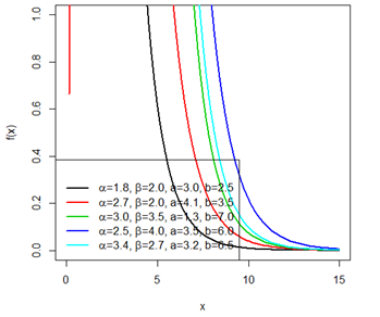
Figure 1 Probability density function of the OGE-IL distribution.

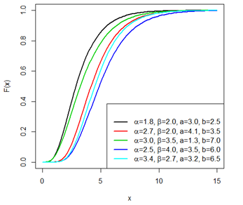
Figure 2 Cumulativve distribution function of the OGE-IL distribution.

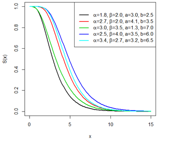
Figure 3 Reliability plot of the OGE-IL distribution.

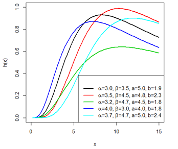
Figure 4 Harzard plot of the OGE-IL distribution.

In this section we derive some of the basic theoretical/structural properties of the OGE-IL distribution, such as; its asymptotic behavior, quantile, median, Skewness and kurtosis of the Odd Generalized Exponentiated Inverse Lomax distribution.

Asymptotic Behavior of the OGE-IL Distribution

We examine the behavior of the OGE-IL distribution in equation (6) as $x\to \infty$ and as  and in equation (10) as i.e. $x\to \infty$

$\underset{x\to 0}{\lim }{f}_{OGE-IL}\left(x\right)=\underset{x\to 0}{lim}\frac{{\displaystyle ab\frac{{\displaystyle \alpha \beta }}{{\displaystyle x^2}}{(1+\frac{{\displaystyle \beta }}{{\displaystyle x}})}^{-(1+\alpha )}}}{{\displaystyle {[1-{(1+\frac{{\displaystyle \beta }}{{\displaystyle x}})}^{-\alpha }]}^2}}{e}^{-b\left(\frac{{\displaystyle {(1+\frac{{\displaystyle \beta }}{{\displaystyle x}})}^{-\alpha }}}{{\displaystyle 1-{(1+\frac{{\displaystyle \beta }}{{\displaystyle x}})}^{-\alpha }}}\right)}{[1-e^{-b\left(\frac{{\displaystyle {(1+\frac{{\displaystyle \beta }}{{\displaystyle x}})}^{-\alpha }}}{{\displaystyle 1-{(1+\frac{{\displaystyle \beta }}{{\displaystyle x}})}^{-\alpha }}}\right)}]}^{a-1}=0$

$\underset{x\to \infty }{lim}{[1-e^{-b\left(\frac{{\displaystyle {(1+\frac{{\displaystyle \beta }}{{\displaystyle x}})}^{-\alpha }}}{{\displaystyle 1-{(1+\frac{{\displaystyle \beta }}{{\displaystyle x}})}^{-\alpha }}}\right)}]}^a=1$

Quantile function and Median

$Q_{OGE-IL}\left(u\right)=F_{OGE-IL}\left(u\right)$

$Let u={[1-e^{-b\left(\frac{{\displaystyle {(1+\frac{{\displaystyle \beta }}{{\displaystyle x}})}^{-\alpha }}}{{\displaystyle 1-{(1+\frac{{\displaystyle \beta }}{{\displaystyle x}})}^{-\alpha }}}\right)}]}^a$

$u^{\raisebox{1ex}{${\displaystyle 1}$}\!\left/ \!\raisebox{-1ex}{${\displaystyle a}$}\right.}=[1-e^{-b\left(\frac{{\displaystyle {(1+\frac{{\displaystyle \beta }}{{\displaystyle x}})}^{-\alpha }}}{{\displaystyle 1-{(1+\frac{{\displaystyle \beta }}{{\displaystyle x}})}^{-\alpha }}}\right)}]$

$1+u^{\raisebox{1ex}{${\displaystyle 1}$}\!\left/ \!\raisebox{-1ex}{${\displaystyle a}$}\right.}=e^{-b\left(\frac{{\displaystyle {(1+\frac{{\displaystyle \beta }}{{\displaystyle x}})}^{-\alpha }}}{{\displaystyle 1-{(1+\frac{{\displaystyle \beta }}{{\displaystyle x}})}^{-\alpha }}}\right)}$

$\ln (1+u^{\raisebox{1ex}{${\displaystyle 1}$}\!\left/ \!\raisebox{-1ex}{${\displaystyle a}$}\right.})=-b\left(\frac{{\displaystyle {(1+\frac{{\displaystyle \beta }}{{\displaystyle x}})}^{-\alpha }}}{{\displaystyle 1-{(1+\frac{{\displaystyle \beta }}{{\displaystyle x}})}^{-\alpha }}}\right)$

$\frac{{\displaystyle -\ln (1+u^{\raisebox{1ex}{${\displaystyle 1}$}\!\left/ \!\raisebox{-1ex}{${\displaystyle a}$}\right.})}}{{\displaystyle b}}=\left(\frac{{\displaystyle {(1+\frac{{\displaystyle \beta }}{{\displaystyle x}})}^{-\alpha }}}{{\displaystyle 1-{(1+\frac{{\displaystyle \beta }}{{\displaystyle x}})}^{-\alpha }}}\right)$

$-\ln (1+u^{\raisebox{1ex}{${\displaystyle 1}$}\!\left/ \!\raisebox{-1ex}{${\displaystyle a}$}\right.})(1-{(1+\frac{{\displaystyle \beta }}{{\displaystyle x}})}^{-\alpha })=b{(1+\frac{{\displaystyle \beta }}{{\displaystyle x}})}^{-\alpha }$

$-\ln (1+u^{\raisebox{1ex}{${\displaystyle 1}$}\!\left/ \!\raisebox{-1ex}{${\displaystyle a}$}\right.})={(1+\frac{{\displaystyle \beta }}{{\displaystyle x}})}^{-\alpha }[b-\ln (1+u^{\raisebox{1ex}{${\displaystyle 1}$}\!\left/ \!\raisebox{-1ex}{${\displaystyle a}$}\right.})]$

$x=\beta {[{\left(\frac{{\displaystyle -\ln (1+u^{\raisebox{1ex}{${\displaystyle 1}$}\!\left/ \!\raisebox{-1ex}{${\displaystyle a}$}\right.})}}{{\displaystyle [b-\ln (1+u^{\raisebox{1ex}{${\displaystyle 1}$}\!\left/ \!\raisebox{-1ex}{${\displaystyle a}$}\right.})]}}\right)}^{\raisebox{1ex}{${\displaystyle -1}$}\!\left/ \!\raisebox{-1ex}{${\displaystyle \alpha }$}\right.}-1]}^{-1}$

$Q\left(u\right)=\beta {\left[{\left(\frac{-\ln \left(1+u^{\raisebox{1ex}{$1$}\!\left/ \!\raisebox{-1ex}{$a$}\right.}\right)}{\left[b-\ln \left(1+u^{\raisebox{1ex}{$1$}\!\left/ \!\raisebox{-1ex}{$a$}\right.}\right)\right]}\right)}^{\raisebox{1ex}{$-1$}\!\left/ \!\raisebox{-1ex}{$\alpha $}\right.}-1\right]}^{-1}$ $Q\left(u\right)=\beta {\left[{\left(\frac{-\ln \left(1+u^{\raisebox{1ex}{$1$}\!\left/ \!\raisebox{-1ex}{$a$}\right.}\right)}{\left[b-\ln \left(1+u^{\raisebox{1ex}{$1$}\!\left/ \!\raisebox{-1ex}{$a$}\right.}\right)\right]}\right)}^{\raisebox{1ex}{$-1$}\!\left/ \!\raisebox{-1ex}{$\alpha $}\right.}-1\right]}^{-1}$ $Q\left(u\right)=\beta {\left[{\left(\frac{-\ln \left(1+u^{\raisebox{1ex}{$1$}\!\left/ \!\raisebox{-1ex}{$a$}\right.}\right)}{\left[b-\ln \left(1+u^{\raisebox{1ex}{$1$}\!\left/ \!\raisebox{-1ex}{$a$}\right.}\right)\right]}\right)}^{\raisebox{1ex}{$-1$}\!\left/ \!\raisebox{-1ex}{$\alpha $}\right.}-1\right]}^{-1}$    (12)

$u~Uniform(0,1)$

$median=\beta {[{\left(\frac{{\displaystyle -\ln (1+{\left(0.5\right)}^{\raisebox{1ex}{${\displaystyle 1}$}\!\left/ \!\raisebox{-1ex}{${\displaystyle a}$}\right.})}}{{\displaystyle [b-\ln (1+{\left(0.5\right)}^{\raisebox{1ex}{${\displaystyle 1}$}\!\left/ \!\raisebox{-1ex}{${\displaystyle a}$}\right.})]}}\right)}^{\raisebox{1ex}{${\displaystyle -1}$}\!\left/ \!\raisebox{-1ex}{${\displaystyle \alpha }$}\right.}-1]}^{-1}$

Skewness and Kurtosis

$S_k=\frac{{\displaystyle q_{\left(0.75\right)}-2q_{\left(0.5\right)}+q_{\left(0.25\right)}}}{{\displaystyle q_{\left(0.75\right)}-q_{\left(0.25\right)}}}$   (13)

$K_u=\frac{{\displaystyle q_{\left(0.875\right)}-q_{\left(0.625\right)}-q_{\left(0.375\right)}+q_{\left(0.125\right)}}}{{\displaystyle q_{\left(0.75\right)}-q_{\left(0.25\right)}}}$   (14)

Moment

${\mu }_r^1=E\left(X^r\right)=\underset{0}{\overset{\infty }{\int }}{x}^r{f}_{OGE-IL}\left(x\right)dx$

${\mu }_r^1=\underset{0}{\overset{\infty }{\int }}\left(x^{r-2}\right)\frac{ab\alpha \beta {(1+\frac{\beta }{x})}^{-(1+\alpha )}}{{[1-{(1+\frac{\beta }{x})}^{-\alpha }]}^2}{e}^{-b\left(\frac{{(1+\frac{\beta }{x})}^{-\alpha }}{1-{(1+\frac{\beta }{x})}^{-\alpha }}\right)}{[1-e^{-b\left(\frac{{(1+\frac{\beta }{x})}^{-\alpha }}{1-{(1+\frac{\beta }{x})}^{-\alpha }}\right)}]}^{a-1}dx$

${\mu }_r^1=ab\alpha \beta \sum _{k=0}^{a-1}\left(\begin{array}{c}a-1\\ k\end{array}\right){(-1)}^k\underset{0}{\overset{\infty }{\int }}\left(x^{r-2}\right)\frac{{(1+\frac{\beta }{x})}^{-(1+\alpha )}}{{[1-{(1+\frac{\beta }{x})}^{-\alpha }]}^2}{e}^{-b(k+1)\left(\frac{{(1+\frac{\beta }{x})}^{-\alpha }}{1-{(1+\frac{\beta }{x})}^{-\alpha }}\right)}dx$

${\mu }_r^1=\sum _{y=0}^{\infty }\sum _{w=0}^{\infty }\sum _{k=0}^{a-1}\left(\begin{array}{c}a-1\\ k\end{array}\right)\left(\begin{array}{c}2-j\\ y\end{array}\right)\frac{{(-1)}^{w+k}{(k+1)}^j}{w!}{\beta }^r\alpha b^{1+w}aB(1-r,\alpha (k+w+y)+r)$    (15)

Order statistics

$f_{j:n}\left(x\right)=\frac{{\displaystyle n!}}{{\displaystyle (j-1)!(n-1)!}}{f}_{OGE-IL}\left(x\right)F_{OGE-IL}{\left(x\right)}^{j-1}{[1-F_{OGE-IL}\left(x\right)]}^{n-j}$

$f_{j:n}\left(x\right)=\frac{{\displaystyle n!}}{{\displaystyle (j-1)!(n-j)!}}\left(\frac{{\displaystyle ab\alpha \beta {(1+\frac{{\displaystyle \beta }}{{\displaystyle x}})}^{-(1+\alpha )}}}{{\displaystyle x^2{[1-{(1+\frac{{\displaystyle \beta }}{{\displaystyle x}})}^{-\alpha }]}^2}}{e}^{-b\left(\frac{{\displaystyle {(1+\frac{{\displaystyle \beta }}{{\displaystyle x}})}^{-\alpha }}}{{\displaystyle 1-{(1+\frac{{\displaystyle \beta }}{{\displaystyle x}})}^{-\alpha }}}\right)}{[1-e^{-b\left(\frac{{\displaystyle {(1+\frac{{\displaystyle \beta }}{{\displaystyle x}})}^{-\alpha }}}{{\displaystyle 1-{(1+\frac{{\displaystyle \beta }}{{\displaystyle x}})}^{-\alpha }}}\right)}]}^{a-1}\right)$

${({[1-e^{-b\left(\frac{{\displaystyle {(1+\frac{{\displaystyle \beta }}{{\displaystyle x}})}^{-\alpha }}}{{\displaystyle 1-{(1+\frac{{\displaystyle \beta }}{{\displaystyle x}})}^{-\alpha }}}\right)}]}^a )}^{j-1}{[1-{[1-e^{-b\left(\frac{{\displaystyle {(1+\frac{{\displaystyle \beta }}{{\displaystyle x}})}^{-\alpha }}}{{\displaystyle 1-{(1+\frac{{\displaystyle \beta }}{{\displaystyle x}})}^{-\alpha }}}\right)}]}^a ]}^{n-j}$  (16)

$f_{1:n}\left(x\right)=n\left(\frac{{\displaystyle ab\alpha \beta {(1+\frac{{\displaystyle \beta }}{{\displaystyle x}})}^{-(1+\alpha )}}}{{\displaystyle x^2{[1-{(1+\frac{{\displaystyle \beta }}{{\displaystyle x}})}^{-\alpha }]}^2}}{e}^{-b\left(\frac{{\displaystyle {(1+\frac{{\displaystyle \beta }}{{\displaystyle x}})}^{-\alpha }}}{{\displaystyle 1-{(1+\frac{{\displaystyle \beta }}{{\displaystyle x}})}^{-\alpha }}}\right)}{[1-e^{-b\left(\frac{{\displaystyle {(1+\frac{{\displaystyle \beta }}{{\displaystyle x}})}^{-\alpha }}}{{\displaystyle 1-{(1+\frac{{\displaystyle \beta }}{{\displaystyle x}})}^{-\alpha }}}\right)}]}^{a-1}\right){[1-{[1-e^{-b\left(\frac{{\displaystyle {(1+\frac{{\displaystyle \beta }}{{\displaystyle x}})}^{-\alpha }}}{{\displaystyle 1-{(1+\frac{{\displaystyle \beta }}{{\displaystyle x}})}^{-\alpha }}}\right)}]}^a ]}^{n-1}$ (17)

$f_{n:n}\left(x\right)=n\left(\frac{{\displaystyle ab\alpha \beta {(1+\frac{{\displaystyle \beta }}{{\displaystyle x}})}^{-(1+\alpha )}}}{{\displaystyle x^2{[1-{(1+\frac{{\displaystyle \beta }}{{\displaystyle x}})}^{-\alpha }]}^2}}{e}^{-b\left(\frac{{\displaystyle {(1+\frac{{\displaystyle \beta }}{{\displaystyle x}})}^{-\alpha }}}{{\displaystyle 1-{(1+\frac{{\displaystyle \beta }}{{\displaystyle x}})}^{-\alpha }}}\right)}{[1-e^{-b\left(\frac{{\displaystyle {(1+\frac{{\displaystyle \beta }}{{\displaystyle x}})}^{-\alpha }}}{{\displaystyle 1-{(1+\frac{{\displaystyle \beta }}{{\displaystyle x}})}^{-\alpha }}}\right)}]}^{a-1}\right){({[1-e^{-b\left(\frac{{\displaystyle {(1+\frac{{\displaystyle \beta }}{{\displaystyle x}})}^{-\alpha }}}{{\displaystyle 1-{(1+\frac{{\displaystyle \beta }}{{\displaystyle x}})}^{-\alpha }}}\right)}]}^a )}^{n-1}$ (18)

Parameter estimation

$L=\prod _{i=1}^{n}f(x_i;\alpha ,\beta ,a,b)$

$L(x_i;\alpha ,\beta ,a,b)=\prod _{i=1}^n\frac{ab\alpha \beta {(1+\frac{\beta }{x})}^{-(1+\alpha )}}{x^2{[1-{(1+\frac{\beta }{x})}^{-\alpha }]}^2}{e}^{-b\left(\frac{{(1+\frac{\beta }{x})}^{-\alpha }}{1-{(1+\frac{\beta }{x})}^{-\alpha }}\right)}{[1-e^{-b\left(\frac{{(1+\frac{\beta }{x})}^{-\alpha }}{1-{(1+\frac{\beta }{x})}^{-\alpha }}\right)}]}^{a-1}$

$L(x_i;\alpha ,\beta ,a,b)=n\ln \alpha +n\ln \beta +n\ln a+n\ln b-2\sum _{i=1}^n\ln x_i-2\sum _{i=1}^n\ln (1-\left({(1+\frac{\beta }{x})}^{-\alpha }\right))$

$-(1+\alpha )\sum _{i=1}^n\ln (1+\frac{\beta }{x_i})-b\sum _{i=1}^n\left(\frac{{(1+\frac{\beta }{x})}^{-\alpha }}{1-{(1+\frac{\beta }{x})}^{-\alpha }}\right)+(a-1)\sum _{i=1}^n\ln (1-e^{-b\left(\frac{{(1+\frac{\beta }{x})}^{-\alpha }}{1-{(1+\frac{\beta }{x})}^{-\alpha }}\right)})$ (19)

$\frac{\partial \ln L\left(x\right)}{\partial \beta }=\frac{n}{\beta }-b\alpha \sum _{i=1}^n\frac{{(1+\frac{\beta }{x})}^{-\alpha }}{{[{(1+\frac{\beta }{x})}^{-\alpha }-1]}^2(x+\beta )}-(1-\alpha )\sum _{i=1}^n{(x+\beta )}^{-1}+\frac{2\alpha {(1+\frac{\beta }{x})}^{-\alpha }}{(x+\beta )[{(1+\frac{\beta }{x})}^{-\alpha }-1]}$

$+b\alpha (a-1)\sum _{i-1}^n\frac{{(1+\frac{\beta }{x})}^{-\alpha }{e}^{-b\left(\frac{{(1+\frac{\beta }{x})}^{-\alpha }}{1-{(1+\frac{\beta }{x})}^{-\alpha }}\right)}}{(x+\beta ){[{(1+\frac{\beta }{x})}^{-\alpha }-1]}^2(1-e^{-b\left(\frac{{(1+\frac{\beta }{x})}^{-\alpha }}{1-{(1+\frac{\beta }{x})}^{-\alpha }}\right)})}=0$ (20)

$\frac{\partial \ln L\left(x\right)}{\partial \beta }=\frac{n}{\alpha }-2\sum _{i=1}^n\frac{{(1+\frac{\beta }{x})}^{-\alpha }\ln (1+\frac{\beta }{x})}{1-{(1+\frac{\beta }{x})}^{-\alpha }}+b\sum _{i=1}^n\frac{{(1+\frac{\beta }{x})}^{-\alpha }\ln (1+\frac{\beta }{x})}{{[{(1+\frac{\beta }{x})}^{-\alpha }-1]}^2(x+\beta )}$

$-\sum _{i=1}^n\ln \ln (1+\frac{\beta }{x})+b(a-1)\sum _{i-1}^n\frac{\ln (1+\frac{\beta }{x}){(1+\frac{\beta }{x})}^{-\alpha }{e}^{-b\left(\frac{{(1+\frac{\beta }{x})}^{-\alpha }}{1-{(1+\frac{\beta }{x})}^{-\alpha }}\right)}}{{[{(1+\frac{\beta }{x})}^{-\alpha }-1]}^2(1-e^{-b\left(\frac{{(1+\frac{\beta }{x})}^{-\alpha }}{1-{(1+\frac{\beta }{x})}^{-\alpha }}\right)})}=0$ (21)

$\frac{\partial \ln L\left(x\right)}{\partial a}=\frac{n}{\alpha }+\sum _{i=1}^n\ln (1-e^{-b\left(\frac{{(1+\frac{\beta }{x})}^{-\alpha }}{1-{(1+\frac{\beta }{x})}^{-\alpha }}\right)})=0$ (22)

$\frac{\partial \ln L\left(x\right)}{\partial b}=\frac{n}{b}-\sum _{i=1}^n(1-e^{-b\left(\frac{{(1+\frac{\beta }{x})}^{-\alpha }}{1-{(1+\frac{\beta }{x})}^{-\alpha }}\right)})+(a-1)\sum _{i=1}^n\left(\frac{-b\left(\frac{{(1+\frac{\beta }{x})}^{-\alpha }}{1-{(1+\frac{\beta }{x})}^{-\alpha }}\right)e^{-b\left(\frac{{(1+\frac{\beta }{x})}^{-\alpha }}{1-{(1+\frac{\beta }{x})}^{-\alpha }}\right)}}{1-e^{-b\left(\frac{{(1+\frac{\beta }{x})}^{-\alpha }}{1-{(1+\frac{\beta }{x})}^{-\alpha }}\right)}}\right)=0$ (23)

Using the Odd Generalized Exponential family of distribution, we have successfully extended the Inverse Lomax distribution from a two parameter to a four parameter distribution. Densities and theoretical characteristics for the proposed OGE-IL distribution have been derived.

None.

The study received no formal support.

The Authors declare that they are no competing interest.

1. Kleiber C, Kotz S. Statistical size distributions in economics and actuarial sciences. New Jersey: John Wiley & Sons; 2003.
2. B Al Zahrani, M Al Sobhi. On parameters estimation of Lomax distribution under general progressive censoring. Journal of Quality and Survival Engineering. 2013.
3. A Hassan, A Al Ghamdi. Optimum step stress accelerated life testing for Lomax distribution. Journal of Applied Sciences Research. 2009;5;2153–2164.
4. SK Singh, U Singh, D Kumar. Bayes estimators of the survival function and parameters of inverted exponential distribution using informative and non–informative priors. Journal of Statistical computation and simulation. 2012;83(12):2258–2269.
5. Yadav AS, Singh SK, Singh U. Bayesian estimation of lomax distribution under type–ii hybrid censored data using lindley’s approximation method. Int Journal of data science. 2016;
6. M Alizadeh, GM Cordeiro, LG Bastos Pinho, et al. The Gompertz–G Family of distributions. Journal of Statistical Theory and Practice. 2017;11(1):179–207.
7. GM Cordeiro, M Alizadeh, ADC Nascimento, et al. The Exponentiated Gompertz generated family of distributions: properties and applications. Chilean Journal of Statistics. 2016;7(2):29–50.
8. Tahir MH, Cordeiro GM, Alizadeh M, et al. The Odd Generalized Exponential Family of Distributions with Applications. Journal of Statistical Distributions and Applications. 2015;2:1–28.
9. Kenney J, Keeping E. Mathematics of Statistics. Volume 1. New Jersey: Princeton University; 1961.
10. Moors JJA. A quantile alternative for kurtosis. Journal of the Royal Statistical Society. 1988;37(1):25–32.