A new three-parameter size-biased poisson-lindley distribution with properties and applications

doi:10.15406/bbij.2020.09.00294

eISSN: 2378-315X

Biometrics & Biostatistics International Journal

Research Article Volume 9 Issue 1

A new three-parameter size-biased poisson-lindley distribution with properties and applications

Rama Shanker,¹

Verify Captcha

Regret for the inconvenience: we are taking measures to prevent fraudulent form submissions by extractors and page crawlers. Please type the correct Captcha word to see email ID.

Kamlesh Kumar Shukla²

¹Department of Statistics, Assam University, India
²Department of Statistics, College of Science, Eritrea

Correspondence: Rama Shanker, Department of Statistics, Assam University, Silchar, India

Received: September 02, 2019 | Published: February 11, 2020

Citation: Shanker R, Shukla KK. A new three-parameter size-biased poisson-lindley distribution with properties and applications. Biom Biostat Int J. 2020;9(1):1-14. DOI: 10.15406/bbij.2020.09.00294

Download PDF

Abstract

A new three-parameter size-biased Poisson-Lindley distribution which includes several one parameter and two-parameter size-biased distributions including size-biased geometric distribution (SBGD), size-biased negative binomial distribution (SBNBD), size-biased Poisson-Lindley distribution (SBPLD), size-biased Poisson-Shanker distribution (SBPSD), size-biased two-parameter Poisson-Lindley distribution-1 (SBTPPLD-1), size-biased two-parameter Poisson-Lindley distribution-2(SBTPPLD-2), size-biased quasi Poisson-Lindley distribution (SBQPLD) and size-biased new quasi Poisson-Lindley distribution (SBNQPLD) for particular cases of parameters has been proposed. Its various statistical properties based on moments including coefficient of variation, skewness, kurtosis and index of dispersion have been studied. Maximum likelihood estimation has been discussed for estimating the parameters of the distribution. Goodness of fit of the proposed distribution has been discussed.

Keywords: three-parameter Lindley distribution, new three-parameter Poisson-Lindley distribution, size-biased distributions, maximum likelihood estimation, goodness of fit

Abbreviations

SBGD, size-biased geometric distribution; SBNBD, size-biased negative binomial distribution; SBPLD, size-biased Poisson-Lindley distribution; SBPSD, size-biased Poisson-Shanker distribution; SBTPPLD-1, size-biased two-parameter Poisson-Lindley distribution-1; SBTPPLD-2, size-biased two-parameter Poisson-Lindley distribution-2; SBQPLD, size-biased quasi Poisson-Lindley distribution; SBNQPLD, size-biased new quasi Poisson-Lindley distribution; ATPLD, A three- parameter Lindley distribution

Introduction

A three- parameter Lindley distribution (ATPLD) introduced by Shanker et al.,¹ is defined by its probability density function (pdf) and cumulative distribution function (cdf)

$f (x; θ, α, β) = \frac{θ^{2}}{θ α + β} (α + β x) e^{- θ x}; x > 0, θ > 0, β > 0, θ α + β > 0$ (1.1)

$F (x; θ, α, β) = 1 - [1 + \frac{θ β x}{θ α + β}] e^{- θ x}; x > 0, θ >, β > 0, θ α + β > 0$ (1.2)

It has been observed that ATPLD is a convex combination of exponential and gamma distributions with mixing proportion $p = \frac{θ α}{θ α + β}$ . Shanker et al.,¹ discussed its statistical properties, estimation of parameters using maximum likelihood estimation and applications to model lifetime data. Further, ATPLD includes several one parameter and two-parameter lifetime distributions for particular values of parameters. The particular distributions of (1.2) are summarized in table 1 along with their pdf and introducers.

Although Lindley distribution was proposed by Lindley,² but various statistical properties of Lindley distribution was studied by Ghitany et al.³ Statistical properties, estimation of parameters and applications of the particular distributions of ATPLD given in table 1 are available in the respective papers.

Parameter Values	Probability density function	Name of the distribution	Introducers (years)
$α = 1, β = 0$	$f (x; θ) = θ e^{- θ x}; x > 0$	Exponential distribution
$α = β = 1$	$f (x; θ) = \frac{θ^{2}}{θ + 1} (1 + x) e^{- θ x}; x > 0$	Lindley distribution	Lindley²
$α = θ, β = 1$	$f (x; θ) = \frac{θ^{2}}{θ^{2} + 1} (θ + x) e^{- θ x}; x > 0$	Shanker distribution	Shanker¹¹
$β = 1$	$f (x; θ, α) = \frac{θ^{2}}{θ α + 1} (α + x) e^{- θ x}; x > 0$	Two-parameter Lindley distribution-1 (TPLD-1)	Shanker and Mishra¹²
$α = 1$	$f (x; θ, β) = \frac{θ^{2}}{θ + β} (1 + β x) e^{- θ x}; x > 0$	Two-parameter Lindley distribution-2 (TPLD-2)	Shanker et al.¹³
$β = θ$	$f (x; θ, α) = \frac{θ}{α + 1} (α + θ x) e^{- θ x}; x > 0$	Quasi Lindley distribution (QLD)	Shanker and Mishra¹⁴
$α = θ$	$f (x; θ, β) = \frac{θ^{2}}{θ^{2} + β} (θ + β x) e^{- θ x}; x > 0$	New Quasi Lindley distribution (NQLD)	Shanker and Amanuel¹⁵

Table 1 Particular continuous distributions for specific values of parameters of ATPLD with probability density function and its introducers (year)

Recently, Das et al.⁴ proposed a new three-parameter Poisson-Lindley distribution (NTPPLD) by mixing Poisson distribution with ATPLD introduced by Shanker et al.¹given in (1.1). The probability mass function of NTPPLD proposed by Das et al.⁴ is given by

$P_{0} (x; θ, α, β) = \frac{θ^{2}}{θ α + β} \frac{β x + (θ α + α + β)}{{(θ + 1)}^{x + 2}}; x = 0, 1, 2, ..., θ > 0, α > 0, θ α + β > 0$ (1.3)

Statistical properties including moments based measures, generating functions, estimation of parameters and applications of the distribution have been discussed by Das et al.⁴

It has been observed that NTPPLD includes several one parameter and two-parameter discrete distributions based on Poisson mixture of lifetime distributions given in table 1. The particular discrete distributions of (1.3) for particular values of parametersare summarized in table 2 along with their probability mass function (pmf) and introducers (year).

Parameter Values	Probability mass function	Name of the distribution	Introducers (years)
$β = 0, α = 1$	$P (X = x) = \frac{θ}{θ + 1} {(\frac{1}{θ + 1})}^{x}; x = 0, 1, 2, ...$	Geometric distribution
$α = 0, β = 1$	$P (X = x) = (x + 1) {(\frac{θ}{θ + 1})}^{2} {(\frac{1}{θ + 1})}^{x}; x = 0, 1, 2, ...$	Negative Binomial distribution	Greenwood and Yule¹⁶
$α = β = 1$	$P (X = x) = \frac{θ^{2} (x + θ + 2)}{{(θ + 1)}^{x + 3}}; x = 0, 1, 2, ...$	Poisson-Lindley distribution (PLD)	Sankaran¹⁷
$α = θ, β = 1$	$P (X = x) = \frac{θ^{2}}{θ^{2} + 1} \cdot \frac{x + (θ^{2} + θ + 1)}{{(θ + 1)}^{x + 2}}; x = 0, 1, 2, ...$	Poisson-Shanker distribution (PSD)	Shanker⁶
$α = 1$	$P (X = x) = \frac{θ^{2}}{θ^{2} + β} \cdot \frac{β x + θ^{2} + θ + β}{{(θ + 1)}^{x + 2}}; x = 0, 1, 2, ...$	Two-parameter Poisson-Lindley distribution-1 (TPPLD-1)	Shanker et al.¹⁸
$β = 1$	$P (X = x) = \frac{θ^{2}}{θ α + 1} \cdot \frac{x + θ α + α + 1}{{(θ + 1)}^{x + 2}}; x = 0, 1, 2, ...$	Two-parameter Poisson-Lindley distribution-2 (TPPLD-2)	Shanker and Mishra¹⁸
$β = θ$	$P (X = x) = \frac{θ}{α + 1} \cdot \frac{θ x + θ α + α + θ}{{(θ + 1)}^{x + 2}}; x = 0, 1, 2, ...$	Quasi Poisson-Lindley distribution (QPLD)	Shanker and Mishra¹⁹
$α = θ$	$P (X = x) = \frac{θ^{2}}{θ^{2} + β} \cdot \frac{β x + θ^{2} + θ + β}{{(θ + 1)}^{x + 2}}; x = 0, 1, 2, ...$	New Quasi Poisson-Lindley distribution (NQPLD)	Shanker and Tekie²⁰

Table 2 Particular discrete distributions for specific values of parameters of NTPPLD with pmf and its introducers (year)

The first four moments about origin and the variance of NTPPLD, obtained by Das et al.,⁴ are given by

μ_{1}^{'} = \frac{θ α + 2 β}{θ (θ α + β)}

μ_{2}^{'} = \frac{θ^{2} α + 2 (α + β) θ + 6 β}{θ^{2} (θ α + β)}

μ_{3}^{'} = \frac{θ^{3} α + 6 (α + β) θ^{2} + 6 (α + 3 β) θ + 24 β}{θ^{3} (θ α + β)}

μ_{4}^{'} = \frac{θ^{4} α + 2 (7 α + β) θ^{3} + 6 (6 α + 7 β) θ^{2} + 24 (α + 6 β) θ + 120 β}{θ^{4} (θ α + β)}

μ_{2} = σ^{2} = \frac{θ^{3} α^{2} + (α + 3 β) θ^{2} α + 2 (2 α + β) θ β + 2 β^{2}}{θ^{2} {(θ α + β)}^{2}}

The main purpose of this paper is to propose a new three-parameter size-biased Poisson-Lindley distribution which includes several one parameter and two-parameter size-biased distributions for particular cases of parameters. Its moments have been derived and various statistical properties based on moments have been studied. Maximum likelihood estimation has been discussed. Goodness of fit of the distribution has been discussed with several count datasets.

A new three-parameter size-biased poisson-lindley distribution

Using the pmf (1.3) and the mean of NTPPLD, a new three-parameter size-biased Poisson-Lindley distribution (NTPSBPLD) can be obtained as

$P_{1} (x; θ, α, β) = \frac{x \cdot P_{0} (x; θ, α, β)}{{μ^{'}}_{1}} = \frac{θ^{3}}{θ α + 2 β} \frac{x (β x + θ α + α + β)}{{(θ + 1)}^{x + 2}}$ (2.1)

; x = 1, 2, 3, .., (θ, α, β) > 0

It can be easily verified that NTPSBPLD contains several one-parameter and two-parameter size-biased distributions including size-biased geometric distribution (SBGD), size-biased negative binomial distribution (SBNBD), size-biased Poisson-Lindley distribution (SBPLD) proposed by Ghitany and Mutairi,⁵ size-biased Poisson-Shanker distribution(SBPSD) proposed by Shanker,⁶ size-biased two-parameter Poisson-Lindley distribution-1 (SBTPPLD-1) introduced by Shanker,⁷ size-biased two-parameter Poisson-Lindley distribution-2 (SBTPPLD-2) suggested by Shanker and Mishra,⁸ size-biased quasi Poisson-Lindley distribution (SBQPLD) proposed by Shanker and Mishra⁹and size-biased new quasi Poisson-Lindley distribution (SBNQPLD) introduced by Shanker et al.,¹⁰ respectively for $(β = 0, α = 1)$ , $(α = 0, β = 1)$ , $(α = β = 1)$ , $(α = θ, β = 1)$ , $(α = 1)$ , $(β = 1)$ , $(β = θ)$ , $(α = θ)$ respectively.

Various characteristics of a distribution are based on their moments and it not easy to derive the moments of NTPSBPLD directly. Therefore, to derive the moments of NTPSBPLD, the pmf of NTPSBPLD can also be obtained as follows:

Let the random variable follows the size-biased Poisson distribution (SBPD) with parameter and pmf

$g (x | λ) = \frac{e^{- λ} λ^{x - 1}}{(x - 1)!}; x = 1, 2, 3, ...,; λ > 0$ (2.2)

Suppose the parameterof SBPD follows the size-biased three-parameter Lindley distribution with pdf

$h (λ; θ) = \frac{θ^{3}}{θ α + 2 β} λ (α + λ β) e^{- θ λ}; λ > 0, (θ, α, β) > 0$ (2.3)

Thus the pmf of NTPSBPLD can be obtained as

$P (X = x) = \int_{0}^{\infty} g (x | λ) \cdot h (λ; θ) d λ$

$= \int_{0}^{\infty} \frac{e^{- λ} λ^{x - 1}}{(x - 1)!} \frac{θ^{3}}{θ α + 2 β} λ (α + λ β) e^{- θ λ} d λ$ (2.4)

= \frac{θ^{3}}{(θ α + 2 β) (x - 1)!} \int_{0}^{\infty} e^{- (θ + 1) λ} λ^{x} (α + λ β) d λ

= \frac{θ^{3}}{(θ α + 2 β) (x - 1)!} [\frac{α Γ (x + 1)}{{(θ + 1)}^{x + 1}} + \frac{β Γ (x + 2)}{{(θ + 1)}^{x + 2}}]

= \frac{θ^{3}}{θ α + 2 β} \frac{β x^{2} + (θ α + α + β) x}{{(θ + 1)}^{x + 2}}; x = 1, 2, 3, .., (θ, α, β) > 0

which is the pmf of NTPSBPLD obtained in (2.1).

The behavior of the pmf of NTPSBPLD for varying values of parameters $(θ, α, β)$ has been shown in Figure 1.

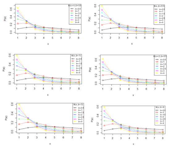
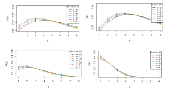
Figure 1 Behavior of NTPSBPLD for $(θ, α, β)$ .

Moments

Using (2.4), the th factorial moment about origin $μ_{(r)}^{'}$ of the NTPSBPLD (2.1) can be obtained as

$μ_{(r)}^{'} = E [E (X^{(r)} | λ)]$ , where $X^{(r)} = X (X - 1) (X - 2) ... (X - r + 1)$

= \int_{0}^{\infty} [\sum_{x = 1}^{\infty} x^{(r)} \frac{e^{- λ} λ^{x - 1}}{(x - 1)!}] \cdot \frac{θ^{3}}{θ α + 2 β} λ (α + λ β) e^{- θ λ} d λ

= \int_{0}^{\infty} [λ^{r - 1} {\sum_{x = r}^{\infty} x \frac{e^{- λ} λ^{x - r}}{(x - r)!}}] \cdot \frac{θ^{3}}{θ α + 2 β} λ (α + λ β) e^{- θ λ} d λ

Taking $y = x - r$ , we get

μ_{(r)}^{'} = \int_{0}^{\infty} [λ^{r - 1} {\sum_{y = 0}^{\infty} (y + r) \frac{e^{- λ} λ^{y}}{y!}}] \cdot \frac{θ^{3}}{θ α + 2 β} λ (α + λ β) e^{- θ λ} d λ

= \frac{θ^{3}}{θ α + 2 β} \int_{0}^{\infty} λ^{r} (λ + r) (α + λ β) e^{- θ λ} d λ

= \frac{θ^{3}}{θ α + 2 β} \int_{0}^{\infty} {β λ^{r + 2} + (α + β r) λ^{r + 1} + r α λ^{r}} e^{- θ λ} d λ

After a little tedious algebraic simplification, the th factorial moment about origin of NTPSBPLD (2.1) can be expressed as

$μ_{(r)}^{'} = \frac{r! {r α θ^{2} + (r + 1) (α + r β) θ + (r + 1) (r + 2) β}}{θ^{r} (θ α + 2 β)}; r = 1, 2, 3, ...$ (3.1)

The first four factorial moments about origin can be obtained by taking $r = 1, 2, 3, and 4$ in (3.1). The first four moments about origin of the NTPSBPLD, using the relationship between moments about origin and factorial moments about origin, are obtained as

μ_{1}^{'} = \frac{α θ^{2} + 2 (α + β) θ + 6 β}{θ (θ α + 2 β)}

μ_{2}^{'} = \frac{α θ^{3} + (6 α + 2 β) θ^{2} + (6 α + 18 β) θ + 24 β}{θ^{2} (θ α + 2 β)}

μ_{3}^{'} = \frac{α θ^{4} + (14 α + 2 β) θ^{3} + (36 α + 42 β) θ^{2} + (24 α + 144 β) θ + 120 β}{θ^{3} (θ α + 2 β)}

μ_{4}^{'} = \frac{α θ^{5} + (30 α + 2 β) θ^{4} + (150 α + 90 β) θ^{3} + (240 α + 600 β) θ^{2} + (120 α + 1200 β) + 720 β}{θ^{4} (θ α + 2 β)}

Now, using the relationship between moments about mean and the moments about origin, the moments about mean of the NTPSBPLD (2.1) can be obtained as

μ_{2} = \frac{2 {α^{2} θ^{3} + (α^{2} + 5 α β) θ^{2} + (6 β^{2} + 6 α β) θ + 6 β^{2}}}{θ^{2} {(θ α + 2 β)}^{2}}

μ_{3} = \frac{2 {\begin{cases} α^{3} θ^{5} + (7 α^{2} β + 3 α^{3}) θ^{4} + (16 α β^{2} + 24 α^{2} β + 2 α^{3}) θ^{3} \\ + (54 α β^{2} + 12 β^{3} + 18 α^{2} β) θ^{2} + (36 α β^{2} + 36 β^{3}) θ + 24 β^{3} \end{cases}}}{θ^{3} {(θ α + 2 β)}^{3}}

μ_{4} = \frac{2 {\begin{cases} α^{4} θ^{7} + (13 α^{4} + 9 α^{3} β) θ^{6} + (30 α^{2} β^{2} + 130 α^{3} β + 24 α^{2}) θ^{5} \\ + (460 α^{2} β^{2} + 44 α β^{3} + 264 α^{3} β + 12 α^{4}) θ^{4} + (936 α^{2} β^{2} + 24 β^{4} + 144 α^{3} β + 696 α β^{3}) θ^{3} \\ + (384 β^{4} + 1368 α β^{3} + 504 α^{2} β^{2}) θ^{2} + (720 β^{4} + 720 α β^{3}) θ + 360 β^{4} \end{cases}}}{θ^{4} {(θ α + 2 β)}^{4}}

The coefficient of variation $(C . V)$ , coefficient of Skewness $(\sqrt{β_{1}})$ , coefficient of Kurtosis $(β_{2})$ and index of dispersion $(γ)$ of the NTPSBPLD (2.1)) are thus obtained as

C . V = \frac{σ}{{μ^{'}}_{1}} = \frac{\sqrt{2 {α^{2} θ^{3} + (α^{2} + 5 α β) θ^{2} + (6 β^{2} + 6 α β) θ + 6 β^{2}}}}{{α θ^{2} + 2 (α + β) θ + 6 β}}

\sqrt{β_{1}} = \frac{μ_{3}}{μ_{2}^{3 / 2}} = \frac{{\begin{cases} α^{3} θ^{5} + (7 α^{2} β + 3 α^{3}) θ^{4} + (16 α β^{2} + 24 α^{2} β + 2 α^{3}) θ^{3} \\ + (54 α β^{2} + 12 β^{3} + 18 α^{2} β) θ^{2} + (36 α β^{2} + 36 β^{3}) θ + 24 β^{3} \end{cases}}}{\sqrt{2} {α^{2} θ^{3} + (α^{2} + 5 α β) θ^{2} + (6 β^{2} + 6 α β) θ + 6 β^{2}}^{3 / 2}}

β_{2} = \frac{μ_{4}}{μ_{2}^{2}} = \frac{{\begin{cases} α^{4} θ^{7} + (13 α^{4} + 9 α^{3} β) θ^{6} + (30 α^{2} β^{2} + 130 α^{3} β + 24 α^{2}) θ^{5} \\ + (460 α^{2} β^{2} + 44 α β^{3} + 264 α^{3} β + 12 α^{4}) θ^{4} + (936 α^{2} β^{2} + 24 β^{4} + 144 α^{3} β + 696 α β^{3}) θ^{3} \\ + (384 β^{4} + 1368 α β^{3} + 504 α^{2} β^{2}) θ^{2} + (720 β^{4} + 720 α β^{3}) θ + 360 β^{4} \end{cases}}}{2 {α^{2} θ^{3} + (α^{2} + 5 α β) θ^{2} + (6 β^{2} + 6 α β) θ + 6 β^{2}}^{2}}

γ = \frac{σ^{2}}{μ_{1}^{'}} = \frac{2 {α^{2} θ^{3} + (α^{2} + 5 α β) θ^{2} + (6 β^{2} + 6 α β) θ + 6 β^{2}}}{θ (θ α + 2 β) {(α θ^{2} + 2 (α + β) θ + 6 β)}}

The graphs of coefficient of variation $(C . V)$ , coefficient of Skewness $(\sqrt{β_{1}})$ , coefficient of Kurtosis $(β_{2})$ and index of dispersion $(γ)$ of the NTPSBPLD are shown in figures 2,3,4 and 5 respectively.

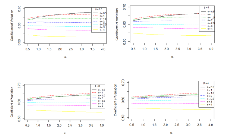
Figure 2 Graphs of coefficient of Variation of the NTPSBPLD for varying values of the parameters $(θ, α, β)$ .

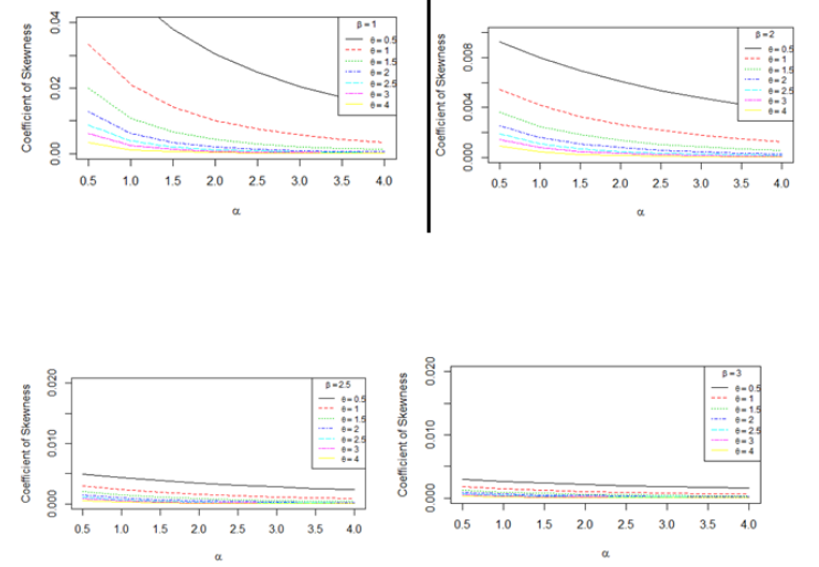
Figure 3 Graphs of coefficient of Skewness of the NTPSBPLD for varying values of the parameters $(θ, α, β)$ .

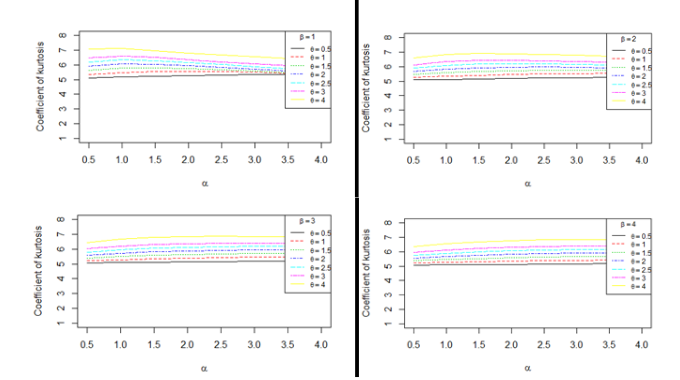
Figure 4 Graphs of Coefficient of Kurtosis of the NTPSBPLD for varying values of the parameter $(θ, α, β)$ .

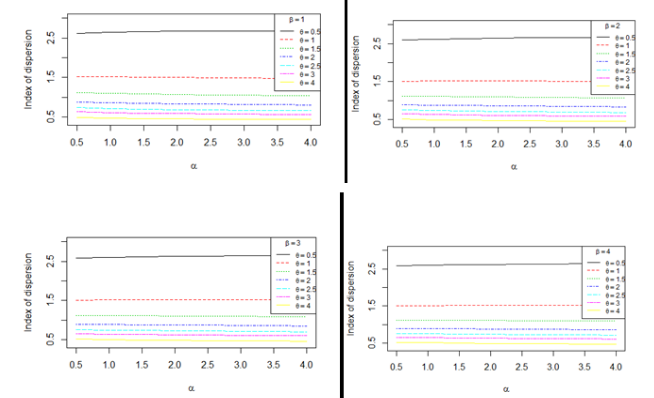
Figure 5 Index of dispersion of the NTPSBPLD for varying values of the parameter $(θ, α, β)$ .

Maximum likelihood estimation

Let us consider $(x_{1}, x_{2}, x_{3}, ..., x_{n})$ as random sample from NTPSBPLD $(θ, α, β)$ . Suppose $f_{x}$ be the observed frequency in the sample corresponding to $X = x (x = 1, 2, 3, ..., k)$ such that $\sum_{x = 1}^{k} f_{x} = n$ , where $k$ is the largest observed value having non-zero frequency. The likelihood function $L$ of NTPSBPLD $(θ, α, β)$ can be expressed as

$L = {(\frac{θ^{3}}{θ α + 2 β})}^{n} \frac{1}{{(θ + 1)}^{\sum_{x = 1}^{k} f_{x} (x + 2)}} Π_{x = 1}^{k} {[β x^{2} + (θ α + α + β) x]}^{f_{x}}$ .

The log likelihood function of NTPSBPLD $(θ, α, β)$ is

\log L = n {3 \log θ - \log (θ α + 2 β)} - \sum_{x = 1}^{k} f_{x} (x + 2) \log (θ + 1) + \sum_{x = 1}^{k} f_{x} \log {β x^{2} + (θ α + α + β) x}

The maximum likelihood estimates, MLE’s $(\hat{θ}, \hat{α}, \hat{β})$ , of parameters $(θ, α, β)$ of NTPSBPLD $(θ, α, β)$ is the solutions of the following log likelihood equations

\frac{\partial \log L}{\partial θ} = \frac{3 n}{θ} - \frac{3 n α}{θ α + 2 β} - \frac{n (\bar{x} + 2)}{θ + 1} + \sum_{x = 1}^{k} \frac{α x f_{x}}{β x^{2} + (θ α + α + β) x} = 0

\frac{\partial \log L}{\partial α} = - \frac{n θ}{θ α + 2 β} + \sum_{x = 1}^{k} \frac{(θ + 1) x f_{x}}{β x^{2} + (θ α + α + β) x} = 0

\frac{\partial \log L}{\partial β} = - \frac{2 n}{θ α + 2 β} + \sum_{x = 1}^{k} \frac{(x^{2} + x) f_{x}}{β x^{2} + (θ α + α + β) x} = 0

where $\bar{x}$ is the sample mean.

Since these log likelihood equations cannot be expressed in closed forms and hence do not seem to be solved directly, the (MLE’s) $(\hat{θ}, \hat{α}, \hat{β})$ of parameters $(θ, α, β)$ can be computed directly by solving the log likelihood equation using R-software till sufficiently close estimates of $(\hat{θ}, \hat{α}, \hat{β})$ are attained.

Goodness of fit

The goodness of fit of NTPSBPLD has been discussed with several count data from various fields of knowledge. The expected frequencies according to the SBPLD, SBQPLD and SBNQPLD using maximum likelihood estimates of parameters have also been given in these tables for ready comparison with those obtained by the NTPSBPLD. Clearly the goodness of fit of NTPSBPLD provides better fit over SBPLD and competing well with SBQPLD and SBNQPLD in majority of datasets. In some of the tables the degree of freedom is zero, and hence p-values have not been given and thus in such tables comparisons can be done on the basis of values of and AIC (Akaike information criterion). The datasets considered for testing the goodness of fit of SBPLD, SBQPLD, SBNQPLD and NTPSBPLD as follows: (Tables i-x)

Group Size	Observed frequency	Expected frequency
Group Size	Observed frequency	SBPLD	SBQPLD	SBNQPLD	NTPSBPLD
1 2 3 4 5 6	1486 694 195 37 10 1	1532.5 630.6 191.9 51.3 12.8 3.9	1485.4 697.2 189.7 41.1 7.8 1.8	1505.5 656.8 202.5 49.2 9.0 0.0	1485.4 697.2 189.7 41.1 7.8
Total	2423	2423.0	2423
ML Estimate		$\hat{θ} = 4.5082$	$\hat{θ} =$ 7.14063 $\hat{α} =$ -0.79104	$\hat{θ} =$ 2.69606 $\hat{α} =$ -1.39128	$\hat{θ} =$ 7.1386 $\hat{α} =$ -0.9318 $\hat{β} = 8.4164$
$χ^{2}$		13.760	0.776	6.1	0.77
d.f.		3	2	2	1
p-value		0.003	0.6804	0.04735	0.3802
$- 2 \log L$		4622.36	4607.8	4610.0	4607.8
AIC		4624.36	4611.8	4614.0	4613.8

Table i Pedestrians-Eugene, Spring, Morning, available in Coleman and James²¹

Group Size	Observed frequency	Expected frequency
Group Size	Observed frequency	SBPLD	SBQPLD	SBNQPLD	NTPSBPLD
1 2 3 4 5	316 141 44 5 4	322.9 132.5 40.2 10.7 3.7	315.7 142.7 40.1 9.1 2.4	313.5 141.4 44.1 10.4 0.6	315.7 142.7 40.1 9.1 2.4
Total	510	510.0	510.0
ML Estimate		$\hat{θ} =$ 4.5211	$\hat{θ} =$ 6.5501 $\hat{α} =$ -0.5069	$\hat{θ} =$ 2.4693 $\hat{α} =$ -1.2977	$\hat{θ} =$ 6.5560 $\hat{α} =$ -0.6029 $\hat{β} = 7.7499$
$χ^{2}$		3.07	0.94	0.38	0.94
d.f.		2	1	1	0
p-value		0.2154	0.3322	0.5376
$- 2 \log L$		972.78	971.07	970.24	971.07
AIC		974.78	975.07	974.24	977.07

Table ii Play Groups-Eugene, spring, Public Playground A, available in Coleman and James²¹

Group Size	Observed frequency	Expected frequency
Group Size	Observed frequency	SBPLD	SBQPLD	SBNQPLD	NTPSBPLD
1 2 3 4 5	306 132 47 10 2	309.4 131.2 41.1 11.3 4.0	304.4 137.9 41.3 10.3 3.1	306.4 134.4 41.6 11.0 3.6	304.4 137.9 41.3 10.3 3.1
Total	497	497.0
ML Estimate		$\hat{θ} = 4.3548$	$\hat{θ} =$ 5.71547 $\hat{α} =$ -0.06947	$\hat{θ} =$ 4.9998 $\hat{α} =$ 25.6948	$\hat{θ} =$ 5.7156 $\hat{α} =$ -0.0708 $\hat{β} = 5.8180$
$χ^{2}$		0.932	1.19	1.2	1.19
d.f.		2	1	1	0
p-value		0.6281	0.2753	0.2733
$- 2 \log L$		971.86	970.96	971.25	970.9
AIC		973.86	974.96	975.25	976.9

Table iii Play Groups-Eugene, spring, Public Playground A, available in Coleman and James²¹

Group Size	Observed frequency	Expected frequency
Group Size	Observed frequency	SBPLD	SBQPLD	SBNQPLD	NTPSBPLD
1 2 3 4 5 6	305 144 50 5 2 1	314.4 134.4 42.5 11.8 3.1 0.8	304.3 148.2 42.3 9.6 1.9 0.7	310.1 138.8 43.1 11.3 2.7 1.0	304.3 148.2 42.3 9.6 1.9 0.7
Total	507	507.0	507.0	507.0
ML Estimate	$\hat{θ} = 4.3179$	$\hat{θ} =$ 6.70804 $\hat{α} =$ -0.74907	$\hat{θ} =$ 6.70804 $\hat{α} =$ -0.74907	$\hat{θ} =$ 5.1516 $\hat{α} =$ 48.6067	$\hat{θ} =$ 6.7082 $\hat{α} =$ -0.8290 $\hat{β} = 7.4234$
$χ^{2}$		6.415	2.96	4.64	2.96
d.f.		2	1	1	0
p-value		0.040	0.0853	0.0312
$- 2 \log L$		993.10	990.02	991.51	990.02
AIC		995.1	994.02	995.51	996.02

Table iv Play Groups-Eugene, Spring, Public Playground D, available in Coleman and James²¹

Group Size	Observed frequency	Expected frequency
Group Size	Observed frequency	SBPLD	SBQPLD	SBNQPLD	NTPSBPLD
1 2 3 4 5	276 229 61 12 3	319.6 166.5 63.8 21.4 9.7	276.0 228.3 61.9 12.2 2.6	313.7 173.1 65.2 20.7 8.3	276.0 228.3 61.9 12.2 2.6
Total	581	581.0	581.0	581.0	581.0
ML Estimate	$\hat{θ} = 4.3179$	$\hat{θ} =$ 3.4359 $\hat{α} =$ -0.74907	$\hat{θ} =$ 8.6724 $\hat{α} = -1.4944$	$\hat{θ} =$ 4.1645 $\hat{α} =$ 61.0287 $\hat{β} = 7.4234$	$\hat{θ} =$ 8.6726 $\hat{α} =$ -2.5854 $\hat{β} = 15.0041$
$χ^{2}$		37.86	0.017	29.6	0.017
d.f.		2	1	1	0
p-value		0.00	0.8962	0.000	0.0000
$- 2 \log L$		1277.42	1238.11	1268.77	1238.11
AIC		1279.42	1242.11	1272.77	1244.11

Table v Play Groups-Eugene, Spring, Public Playground D, available in Coleman and James²¹

No. of sites with particles	Observed Frequency	Expected Frequency
No. of sites with particles	Observed Frequency	SBPLD	SBQPLD	SBNQPLD	NTPSBPLD
1 2 3 4 5	122 50 18 4 4	119.0 53.8 18.0 $\begin{array}{l} 5.3 \\ 1.9 \end{array}}$	119.2 53.5 17.9 5.3 2.1	119.3 53.3 17.8 5.3 2.3	119.3 53.3 17.8 5.3 2.3
Total	198	198.0	198.0	198.0	198.0
ML estimate		$\hat{θ} = 4.050987$	$\hat{θ} =$ 3.7564 $\hat{α} =$ 10.1281	$\hat{θ} =$ 3.4795 $\hat{α} =$ 0.0216	$\hat{θ} =$ 3.4737 $\hat{α} =$ 1.3965 $\hat{β} = 0.0001$
$χ^{2}$		0.43	0.34	0.28	0.28
d.f.		2	1	1	0
p-value		0.8065	0.5598	0.5967
$- 2 \log L$		409.28	409.17	409.13	409.13
AIC		411.28	413.17	413.13	415.13

Table vi Distribution of number of counts of sites with particles from Immunogold data, available in Mathews and Appleton²²

No. times hares caught	Observed Frequency	Expected Frequency
No. times hares caught	Observed Frequency	SBPLD	SBQPLD	SBNQPLD	NTPSBPLD
1 2 3 4 5	184 55 14 4 4	177.3 62.5 $\begin{array}{l} 16.4 \\ 3.8 \\ 1.0 \end{array}}$	177.4 62.3 16.3 3.8 1.2	177.5 62.2 16.3 3.8 1.2	177.5 62.2 16.3 3.8 1.2
Total	261	261.0	261	261.0
ML estimate		$\hat{θ} = 5.351256$	$\hat{θ} =$ 4.9800 $\hat{α} =$ 14.9193	$\hat{θ} =$ 4.6959 $\hat{α} =$ -0.0302	$\hat{θ} =$ 4.6994 $\hat{α} =$ 12.0044 $\hat{β} = - 0.0390$
$χ^{2}$		1.18	3.2	3.19	3.19
d.f.		1	1	1	0
p-value		0.2773	0.0736	0.07409
$- 2 \log L$		457.10	456.86	456.80	456.80
AIC		459.10	460.86	460.80	462.80

Table vii Distribution of snowshoe hares captured over 7 days, available in Keith and Meslow²³

Number of pairs of running shoes	Observed frequency	Expected Frequency
Number of pairs of running shoes	Observed frequency	SBPLD	SBQPLD	SBNQPLD	NTPSBPLD
1	18	20.3	17.4	19.5	17.4
2	18	17.4	19.6	18.0	19.6
3	12	10.9	12.3	11.3	12.3
4 5	7 5	5.9 5.5	6.1 4.6	6.0 5.2	6.1 4.6
Total	60	60.0	60.0	60	60
ML Estimate		$\hat{θ} = 1.818978$	$\hat{θ} =$ 2.5858 $\hat{α} =$ -0.7318	$\hat{θ} =$ 2.08739 $\hat{α} =$ 17.3228	$\hat{θ} =$ 2.5870 $\hat{α} =$ -0.4739 $\hat{β} = 1.6732$
$χ^{2}$		0.64	0.31	0.33	0.31
d.f.		3	1	2	0
P-value		0.8872	0.5777	0.8478
$- 2 \log L$		187.08	185.55	186.33	185.55
AIC		189.08	189.55	190.33	191.55

Table viii Number of counts of pairs of running shoes owned by 60 members of an athletics club, reported by Simonoff²⁴

Number of fly eggs	Observed Frequency	Expected Frequency
Number of fly eggs	Observed Frequency	SBPLD	SBQPLD	SBNQPLD	NTPSBPLD
1 2 3 4 5 6 7 8 9	22 18 18 11 9 6 3 0 1	20.3 22.0 17.2 11.6 7.2 4.2 2.4 1.3 1.8	19.8 22.1 17.5 11.8 7.3 4.2 2.3 1.3 1.7	19.8 22.1 17.5 11.8 7.3 4.2 2.3 1.3 1.7	19.8 22.1 17.5 11.8 7.3 4.2 2.3 1.3 1.7
Total	88		88.0	88.0	88.0
ML estimate		$\hat{θ} =$ 1.2822	$\hat{θ} =$ 1.3483 $\hat{α} =$ 0.6925	$\hat{θ} =$ 1.3465 $\hat{α} =$ 2.5654	$\hat{θ} =$ 1.4477 $\hat{α} =$ 0.4315 $\hat{β} = 1.3594$
$χ^{2}$		1.39	1.49	1.49	1.49
d.f.		4	3	3	3
p-value		0.8459	0.6845	0.6845	0.6845
$- 2 \log L$		329.92	329.86	329.86	329.86
AIC		331.92	333.86	333.86	335.86

Table ix The numbers of counts of flower heads as per the number of fly eggs reported by Finney and Varley²⁵

$X$	Observed frequency	Expected frequency
$X$	Observed frequency	SBPLD	SBQPLD	SBNQPLD	NTPSBPLD
1	375	262.8	363.3	363.6	363.6
2	143	157.4	156.5	156.3	156.3
3	49	50.4	50.4	50.4	50.4
4 5 6 7 8	17 2 2 1 1	14.2 3.7 0.9 0.2 0.3	14.4 3.9 1.0 0.2 0.4	14.4 3.8 1.0 0.2 0.3	14.4 3.8 1.0 0.2 0.3
Total	590	590.0	590.0	590.0	590.0
ML Estimate		$\hat{θ} =$ 4.24	$\hat{θ} =$ 3.8386 $\hat{α} =$ 17.2968	$\hat{θ} =$ 3.6534 $\hat{α} =$ 0.00067	$\hat{θ} =$ 3.6504 $\hat{α} =$ 12.9869 $\hat{β} = - 0.0377$
$χ^{2}$		2.48	2.11	2.08	2.08
d.f.		3	2	2	1
P-value		0.4789	0.3481	0.3534	0.1492
$- 2 \log L$		1190.4	1189.67	1189.57	1189.57
AIC		1192.4	1193.67	1193.57	1193.57

Table x Number of households having at least one migrant according to the number of observed migrants, reported by Singh and Yadav²⁶

Conclusion

A new three-parameter size-biased Poisson-Lindley distribution which includes several size-biased distributions including size-biased geometric distribution (SBGD), size-biased negative binomial distribution (SBNBD), size-biased Poisson-Lindley distribution (SBPLD), size-biased Poisson-Shanker distribution (SBPSD), size-biased two-parameter Poisson-Lindley distribution-1 (SBTPPLD-1), size-biased two-parameter Poisson-Lindley distribution-2 (SBTPPLD-2), size-biased quasi Poisson-Lindley distribution (SBQPLD) and size-biased new quasi Poisson-Lindley distribution (SBNQPLD) for particular values of parameters has been proposed. Its coefficient of variation, skewness, kurtosis and index of dispersion has been studied. Estimation of parameters has been discussed using maximum likelihood. Goodness of fit of the proposed distribution has been discussed with several count datasets.

References

- Shanker R, Shukla KK, Shanker R, et al. A three–parameter lindley distribution. American Journal of Mathematics and Statistics. 2017;7(1):15–26.
- Lindley DV. Fiducial distributions and Bayes’ theorem. Journal of the Royal Statistical Society, Series B. 1958;20:102–107.
- Ghitany ME, Atieh B, Nadarajah S. Lindley distribution and its application. Mathematics Computing and Simulation. 2008;78:493–506.
- Das KK, Ahmad J, Bhattacharjee S. A new three–parameter poisson–lindley distribution for modeling over dispersed count data, International journal of Applied Engineering Research. 2018;13(25):16468–16477.
- Ghitany ME, Al–Mutairi DK. Size–biased poisson–lindley distribution and its applications, Metron. 2008; LXVI(3):299–311.
- Shanker R. A Size–biased poisson–shanker distribution and its applications. International Journal of Probability and Statistics, 2017;6(3):33–44.
- Shanker R. Size–biased discrete two parameters poisson–lindley distribution and its applications, Global Journal of Pure and Applied Mathematics. 2013;9(4):325–334.
- Shanker R, Mishra A. On size–biased two–parameter poisson–lindley distribution and its applications. American Journal of Mathematics and Statistics. 2017;7(3):99–107.
- Shanker R, Mishra A. on a size–biased quasi poisson lindley distribution, International Journal of Probability and Statistics. 2013b;2(2):28–34.
- Shanker R, Shanker R, Tekie AL, et al. Size–biased new quasi poisson lindley distribution and its applications, International Journal of Statistics and Systems. 2014; 9(2):109–118.
- Shanker R. Shanker Distribution and Its Applications. International Journal of Statistics and Applications. 2015;5(6):338–348.
- Shanker R, Mishra A. A two–parameter Lindley distribution, Statistics in Transition–new series. 2013a;14(1):45–56.
- Shanker R, Sharma S, Shanker R. A two–parameter Lindley distribution for modeling waiting and survival times data. Applied Mathematics. 2013;4(2):363–368.
- Shanker R, Mishra A. A quasi lindley distribution. African Journal of Mathematics and Computer Science Research. 6(4):64–71.
- Shanker R, Amanuel AG. A new quasi lindley distribution, International Journal of Statistics and Systems. 2013;8(2):143–156.
- Greenwood M, Yule Udny G. An Inquiry into the nature of frequency distributions representative of multiple happenings with particular reference to the occurrence of multiple attacks of disease or of repeated accidents. Journal of the Royal Statistical Society. 1920;83(2):255–279.
- Sankaran M. The discrete Poisson–Lindley distribution, Biometrics. 1970;26(1):145–149.
- Shanker R, Mishra A. A two–parameter poisson–lindley distribution, International Journal of Statistics and Systems. 2014;9(1):79–85.
- Shanker R, Mishra A. A quasi Poisson– Lindley distribution. Journal of 2014. Indian Statistical Association. 2016;54(1&2):113–125.
- Shanker R, Tekie AL. A new quasi Poisson–Lindley distribution, International Journal of Statistics and Systems. 2014;9(1):79 –85.
- Coleman JS, James J. The equilibrium size distribution of freely forming groups. Sociometry, 1961;24:36–45.
- Mathews JNS, Appleton DR. An application of the truncated Poisson distribution to Immunogold assay. Biometrics. 1993;49(2):617–621.
- Keith LB, Meslow EC. Trap response by snowshoe hares. Journal of Wildlife Management. 1968;32(4):795–801.
- Simonoff JS. Analyzing Categorical Data, New York Springer. 2003.
- Finney DJ, Varley GC. An example of the truncated Poisson distribution, Biometrics, 1955;11(3):387–394.
- Singh SN, Yadav RC. Trends in rural out–migration at household level. Rural Demogr. 1971;8(1):53–61.
©2020 Shanker, et al. This is an open access article distributed under the terms of the,
which
permits unrestricted use, distribution, and build upon your work non-commercially.