Research Article Volume 7 Issue 4
A generalized Aradhana distribution with properties and applications
Daniel Welday, Rama Shanker
College of Science, Eritrea Institute of Technology, Eritrea
Correspondence: Rama Shanker, College of Science, Eritrea Institute of Technology, Asmara, Eritrea
Received: August 13, 2018 | Published: August 29, 2018
Citation: Welday D, Shanker R. A generalized Aradhana distribution with properties and applications. Biom Biostat Int J. 2018;7(4):374-385. DOI: 10.15406/bbij.2018.07.00234
Download PDF
Abstract
A two-parameter generalized Aradhana distribution which includes one parameter exponential and Aradhana distributions as special cases has been proposed. Its statistical properties including shapes of probability density function for varying values of parameters, coefficient of variation, skeweness, kurtosis, index of dispersion, hazard rate function, mean residual life function, stochastic ordering, mean deviations, Bonferroni and Lorenz curves and stress-strength reliability have been discussed. Maximum likelihood estimation has been discussed for estimating the parameters of the distribution. Applications of the distribution have been explained with two real life time data.
Keywords: aradhana distribution, statistical properties, maximum likelihood estimation, applications
Introduction
In almost every fields of knowledge including engineering, biomedical science, social science, insurance, finance, etc, the statistical analysis and modeling of real life time data are crucial for researchers and policy makers. The classical one parameter life time distributions, namely exponential and Lindley, introduced by Lindley,1 are not always suitable due to theoretical or applied point of view for real lifetime data. To overcome the shortcomings of these classical one parameter distributions and have a better lifetime distribution, a number of one parameter lifetime distributions have been introduced in statistics literature and the statistics literature is flooded with a number of one parameter life time distributions. Shanker2 has introduced a one parameter lifetime distribution named Aradhana distribution having scale parameter q and defined by its probability density function (pdf) and cumulative distribution function (cdf)
(1.1)
(1.2)
The rth raw moments (moments about origin),
of Aradhana distribution obtained by Shanker2 is given by
Thus, the first four raw moments of Aradhana distribution are obtained as
Using the relationship between central moments (moments about mean) and the raw moments, the central moments of Aradhana distribution are given by
Shanker2 has discussed various statistical properties based on moments including coefficient of variation, skewness, kurtosis, index of dispersion, hazard rate function, mean residual life function, stochastic ordering, mean deviation, Bonferoni and Lorenz curves, stress-strength reliability along with estimation of parameter and applications of Aradhana distribution for modeling real lifetime data from engineering and biomedical sciences. A discrete Poisson-Aradhana distribution, a Poisson mixture of Aradhana distribution, has been obtained by Shanker and its statistical properties, estimation of parameter along with applications to model count data are available in Shanker . The Lindley distribution is defined by its pdf and cdf
(1.3)
(1.4)
Ghitany et al.,4 have detailed study on statistical properties, estimation of parameter and application of Lindley distribution for modeling waiting time data in a bank. Shanker et al.,5 have critical and comparative study on modeling of real lifetime data from biomedical sciences and engineering and observed that there are several lifetime data where exponential distribution gives much better fit than Lindley distribution. Recently, Berhane & Shanker6 proposed a discrete Lindley distribution using infinite series approach of discretization and studied its various statistical properties, estimation of parameter and applications.
In this paper a two -parameter generalized Aradhana distribution (GAD) has been proposed which includes exponential and Aradhana distributions. GAD has been found to be more general in nature and wider in scope and possess tremendous capacity to fit observed real lifetime data. Its moments and moments based measures have been obtained and discussed. Statistical properties including hazard rate function, mean residual life function, stochastic ordering, mean deviation, Bonferroni and Lorenz curves and stress -strength parameter of GAD have been discussed. Estimation of parameters has been discussed using the method of maximum likelihood. Applications of the distribution have been explained with two real lifetime data and the fit has been compared with one parameter exponential, Lindley and Aradhana distributions and a generalization of Sujatha distribution (AGSD), proposed by Shanker et al.7
A generalized Aradhana distribution
A generalized Aradhana distribution (GAD) having parameters and
is defined by its pdf and cdf
(2.1)
(2.2)
Note that exponential distribution and Aradhana distribution are special cases of GAD for and, respectively. Further, Like Aradhana distribution, GAD is also a three-component mixture of exponential, gamma and distributions. That is
(2.3)
where
The nature of the pdf and the cdf of GAD for various combinations of the parameters
presented in Figure 1 & Figure 2, respectively.
Statistical properties of GAD
Moments and moments based measures
The rth raw moment, , of GAD can be obtained as
The first four raw moments of GAD are given by
.
The central moments of GAD (2.1) are thus obtained as
The expressions for various coefficients including coefficient of variation, skewness, kurtosis and index of dispersion of GAD are obtained as
The behaviors of C.V, skewness, kurtosis and index of dispersion
of GAD for various combination of parameters and have been presented in Tables 1-4, respectively.
q α |
0.1 |
0.2 |
0.5 |
1 |
2 |
3 |
4 |
5 |
0.1 |
0.755 |
0.8535 |
0.9519 |
0.9843 |
0.9955 |
0.9979 |
0.9988 |
0.9992 |
0.2 |
0.6755 |
0.7552 |
0.8831 |
0.9519 |
0.9843 |
0.9924 |
0.9955 |
0.997 |
0.5 |
0.6172 |
0.6568 |
0.7551 |
0.8534 |
0.9341 |
0.9635 |
0.9771 |
0.984 |
1 |
0.597 |
0.6173 |
0.6756 |
0.7551 |
0.8535 |
0.9049 |
0.9341 |
0.952 |
2 |
0.587 |
0.5971 |
0.6273 |
0.6756 |
0.7552 |
0.8125 |
0.8535 |
0.833 |
3 |
0.583 |
0.5904 |
0.6105 |
0.6439 |
0.7048 |
0.7551 |
0.7955 |
0.8277 |
4 |
0.582 |
0.5871 |
0.6021 |
0.6273 |
0.6756 |
0.7184 |
0.7551 |
0.7863 |
5 |
0.581 |
0.5851 |
0.5971 |
0.6105 |
0.6568 |
0.6934 |
0.7262 |
0.755 |
Table 1 C.V of GAD for varying values of parameters and
q α |
0.1 |
0.2 |
0.5 |
1 |
2 |
3 |
4 |
5 |
0.1 |
1.2981 |
1.5314 |
2.0638 |
2.5955 |
3.1058 |
3.3467 |
3.4859 |
3.5763 |
0.2 |
1.1932 |
1.2981 |
1.6376 |
2.0639 |
2.5955 |
2.9057 |
3.1058 |
3.2448 |
0.5 |
1.1589 |
1.1781 |
1.2981 |
1.5313 |
1.9114 |
2.1974 |
2.4194 |
2.5955 |
1 |
1.1553 |
1.1589 |
1.1932 |
1.2981 |
1.5314 |
1.7358 |
1.9114 |
2.0639 |
2 |
1.1548 |
1.1553 |
1.1622 |
1.1932 |
1.2981 |
1.417 |
1.5314 |
1.6376 |
3 |
1.1547 |
1.1549 |
1.1573 |
1.17 |
1.224 |
1.2981 |
1.3775 |
1.456 |
4 |
1.1547 |
1.1548 |
1.1559 |
1.1622 |
1.1932 |
1.2414 |
1.2981 |
1.3576 |
5 |
1.1547 |
1.1547 |
1.1553 |
1.1589 |
1.1781 |
1.211 |
1.2523 |
1.2981 |
Table 2 of GAD for varying values of parameters and
q α |
0.1 |
0.2 |
0.5 |
1 |
2 |
3 |
4 |
5 |
0.1 |
5.3806 |
6.1353 |
7.163 |
8.4341 |
8.8155 |
8.9103 |
8.9473 |
8.9654 |
0.2 |
5.0871 |
5.3806 |
6.4784 |
7.613 |
8.4341 |
8.7 |
8.8155 |
8.8754 |
0.5 |
5.0082 |
5.0507 |
5.3806 |
6.1353 |
7.26 |
7.8744 |
8.2225 |
8.4341 |
1 |
5.0012 |
5.0082 |
5.0871 |
5.3806 |
6.1353 |
6.779 |
7.2601 |
7.613 |
2 |
5.0002 |
5.0012 |
5.0151 |
5.087 |
5.3806 |
5.7583 |
6.1353 |
6.4784 |
3 |
5.0001 |
5.0004 |
5.005 |
5.032 |
5.1673 |
5.3806 |
5.6297 |
5.8864 |
4 |
5.00002 |
5.0002 |
5.0022 |
5.015 |
5.0871 |
5.2151 |
5.3806 |
5.5659 |
5 |
5.00001 |
5.0001 |
5.0012 |
5.0082 |
5.0507 |
5.1325 |
5.2459 |
5.3806 |
Table 3 Amplitude in mill volts of the Lead-1 of electrocardiography in sheep
*Significant (P≤0.05); NSNot significant (P>0.05)
q α |
0.1 |
0.2 |
0.5 |
1 |
2 |
3 |
4 |
5 |
0.1 |
12.5454 |
6.5556 |
2.4981 |
1.1594 |
0.5449 |
0.354 |
0.2619 |
0.2077 |
0.2 |
11.5851 |
6.2727 |
2.619 |
1.2491 |
0.5797 |
0.3717 |
0.2724 |
0.2147 |
0.5 |
10.6807 |
5.6548 |
2.509 |
1.3111 |
0.6377 |
0.4085 |
0.2969 |
0.2319 |
1 |
10.3402 |
5.3403 |
2.317 |
1.2545 |
0.6556 |
0.4336 |
0.3189 |
0.2498 |
2 |
10.1689 |
5.1701 |
2.1692 |
1.1585 |
0.6273 |
0.4325 |
0.3278 |
0.2619 |
3 |
10.1122 |
5.1129 |
2.1136 |
1.111 |
0.599 |
0.4182 |
0.3219 |
0.261 |
4 |
10.084 |
5.0844 |
2.0852 |
1.0846 |
0.5793 |
0.4049 |
0.3136 |
0.2562 |
5 |
10.067 |
5.0674 |
2.068 |
1.0681 |
0.5655 |
0.3944 |
0.306 |
0.2509 |
Table 4 of GAD for varying values of parameters and
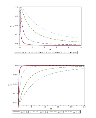
For a fixed value of α, C.V increases as the value of increases. Again for a fixed value of , C.V decrease as the value of increases.
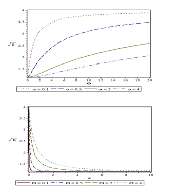
Clearly for any given values of parameters and , coefficient of skewness is always positive and this means that it is always positively skewed.
Since
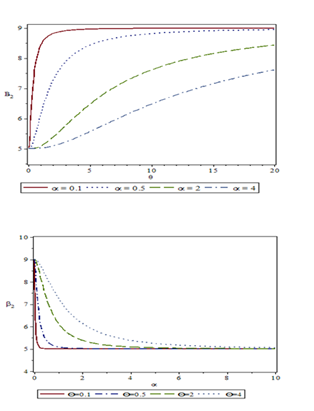
GAD is always leptokurtic, which means that GAD is more peaked than the normal curve
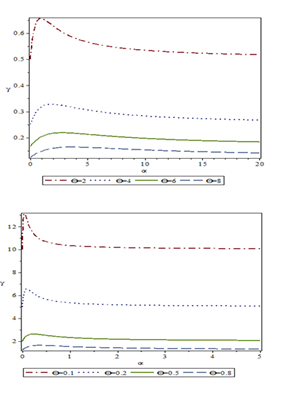
As long as
, GAD is over dispersed and for
, GAD is under-dispersed. The nature of C.V,,and of GAD for various combinations of parameters and have been shown graphically in Figures 3-6, respectively.

Figure 3 Coefficient of variation of GAD for different values of parameters and .

Figure 4Coefficient of Skewness of GAD for different values of parameters and .

Figure 5Coefficient of kurtosis of GAD for different values of parameters and .

Figure 6Index of dispersion of GAD for different values of parameters and .
Hazard rate function and mean residual life function
The hazard rate function (also known as the failure rate function)  and the mean residual life function
  of a continuous random variable
 having pdf
  and cdf
  are respectively defined as
and
Thus, GAD are thus obtained as
and
It can be easily verified that
and
. The behaviors of and of GAD for various combinations of parameters and have been shown graphically in Figure 7 & Figure 8, respectively. Clearly is monotonically increasing whereas
is monotonically decreasing.
Stochastic orderings
Stochastic ordering of positive continuous random variables is very much useful for judging their comparative behavior. A random variable
is said to be smaller than a random variable y in the
- stochastic order
if
for all x
- hazard rate order
if
for all x
- mean residual life order
for all x
- likelihood ratio order
if
decreases in x.
The following interrelationship among various stochastic orderings due to Shaker & Shanthikumar8 are well known for establishing stochastic ordering of distributions
Theorem: Let x GAD
and


GAD

. If
(or
), then
and hence
, and
.
Proof: We have
Now
This gives
. Thus if
or  ,
.
,
.
This means that
and hence
,  and
and . Thus, GAD is ordered with respect to the strongest ‘likelihood ratio ordering’
Deviations from the Mean and the Median
The mean deviation about the mean,  and the mean deviation about the median,
  are defined as
and
, respectively, where
and . These expressions can be further simplified as
(3.4.1)
and
(3.4.2)
Using pdf (2.1) and the mean of GAD, we get
(3.4.3)
(3.4.4)
Using expressions from (3.4.1), (3.4.2), (3.4.3), and (3.4.4), and
of GAD are
(3.4.5)
(3.4.6)
Bonferroni and lorenz curves and indices
The Bonferroni and Lorenz curves are proposed by Bonferroni9 which are used in economics to study income and poverty and other fields of knowledge including reliability, demography, insurance and medicine, some among others. The Bonferroni and Lorenz curves are defined as
(3.5.1)
and (3.5.2)
The Bonferroni and Gini indices are further simplified as
(3.5.3)
and
(3.5.4)
Using pdf of GAD (2.1), we get
(3.5.5)
Now using equation (3.5.5) in (3.5.1) and (3.5.2), we get
(3.5.6)
and
(3.5.7)
Now using equations (3.5.6) and (3.5.7) in (3.5.3) and (3.5.4), we have
(3.5.8)
(3.5.9)
Stress-strength parameter
Suppose is the random strength and be the random stress of a component. , the component fails instantly and the component will function satisfactorily till . Therefore, is a measure of component reliability and in statistics it is known as stress-strength parameter. It has applications in almost all areas of knowledge including medical science, sociology, psychology, and engineering, some among others.
Let be independent strength and stress random variables having GAD (2.1) having parameters and respectively. Then the stress-strength reliability of GAD (2.1) can be obtained as
Clearly at
and
, the above expression reduces to the corresponding expression of R for Aradhana and exponential distributions.
Parameter estimation
In this section maximum likelihood estimation of parameters of GAD has been discussed. Suppose
be a random sample from GAD (2.1)). The natural log likelihood function is thus obtained as
where x is the sample mean.
The maximum likelihood estimates (MLE)
of parameters
are the solutions of the following non-linear log likelihood equations
It is difficult to solve these two natural log likelihood equations directly because they are not in closed forms. But these equations can be solved using Fisher’s scoring method. For, we have
The solution of following equations gives MLE’s
of
of GAD
where
and
are the initial values of
and
, respectively. These equations are solved iteratively till sufficiently close values of
and
are obtained.
Applications
The goodness of fit of GAD using maximum likelihood estimates has been discussed with two real lifetime dataset and the fit has been compared with exponential, Lindley and Aradhana distributions and a generalization of Sujatha distribution (AGSD) proposed by Shanker et al.7 It has been observed that GAD is more suitable to positively skewed lifetime data. In general, majority of the real lifetime datasets in medical science and engineering are positively skewed and hence GAD is suitable for positively skewed data in these fields of knowledge. Since GAD is a new distribution, still more research is required to find several applications of the distribution in various fields of knowledge. The real lifetime datasets which are positively skewed are as follows
Data set 1: This data represents the lifetime's data relating to relief times (in minutes) of 20 patients receiving an analgesic and reported by Gross & Clark.10
1.1 1.4 1.3 1.7 1.9 1.8 1.6 2.2 1.7 2.7 4.1 1.8
1.5 1.2 1.4 3 1.7 2.3 1.6 2
Data set 2: This data set is the strength data of glass of the aircraft window reported by Fuller et al.11
18.830 20.800 21.657 23.030 23.230 24.050 24.321 25.500
25.520 25.800 26.690 26.770 26.780 27.050 27.670 29.900
31.110 33.200 33.730 33.760 33.890 34.760 35.750 35.910
36.980 37.080 37.090 39.580 44.045 45.29 45.381
For comparing the goodness of fit of GAD, AGSD, Aradhana, Lindley and exponential distributions, values of -2ln L , AIC (Akaike Information Criterion), kolmogorove-Smirnov Statistics (K-S Statistics) and p value of these distributions for two real lifetime datasets have been computed and presented in Table 5. Since the best fit of the distribution corresponds to the lower values of -2ln L, AIC, K-S statistics, it is obvious from table 5 that GAD provides better fit than exponential, Lindley, Aradhana and AGSD.
Conclusion
A generalized Aradhana distribution (GAD) has been introduced which includes both Aradhana distribution proposed by Shanker2 and Lindley distribution proposed by Lindley1as particular cases. The nature of probability density function and cumulative distribution function of GAD has been studied. The raw moments and central moments of the distribution have been obtained and behavior of coefficient of variation, coefficient of skewness, coefficient of kurtosis and index of dispersion of GAD have been studied with varying values of the parameters. Hazard rate function and mean residual life function have been studied with varying values of the parameters. The stochastic ordering, mean deviations, Bonferroni and Lorenz curves, and stress-strength reliability have also been discussed. The method of maximum likelihood has been discussed for estimating parameters. Two examples of real lifetime, one from medical science and one from engineering, have been presented to show the applications and goodness of fit of GAD over exponential, Lindley and Aradhana distributions and AGSD and it has been observed that GAD gives much better fit.
Acknowledgements
Conflict of interests
The author declares there is no conflict of interest.
References
- Lindley DV. Fuducial distribution and Bayes theorem. Journal of the Royal statistical Society. Series B, 1958;20(1):102–107.
- Shanker R. Aradhana distribution and its Applications. International Journal of Statistics and Applications. 2016;6(1):23–34.
- Shanker R. The discrete Poisson–Aradhana distribution. Turkiye Klinikleri Journal of Biostatistics, 2017;9(1):12–22.
- Ghitany ME, Atieh B, Nadarajah S. Lindley distribution and its application, Mathematics and computers in simulation. 2008;78(4):493–506.
- Shanker R, Hagos F, Sujatha S. On modeling of lifetime’s data using exponential and Lindley distributions. Biometrics & Biostatistics International Journal, 2015;2(5):1–9.
- Berhane A, Shanker R. A discrete Lindley distribution with Applications in Biological Sciences. Biometrics and Biostatistics International Journal, 2018;7(2):1–5.
- Shanker R, Shukla KK, Hagos F. A Generalization of Sujatha distribution and its Applications to Real lifetime data. Journal of Institute of Science and Technology (JIST). 2017;22(1):77–94.
- Shaked M, Shanthikumar JG. Stochastic Orders and Their Applications. Academic Press, New York. 1994;37(3).
- Bonferroni CE. Elementi di Statistca generale. Seeber, Firenze.1930.
- Gross AJ. Clark VA. Survival Distributions: Reliability Applications in the Biometrical Sciences. John Wiley, New York. 1975.
- Fuller EJ, Frieman S, Quinn J, et al. Fracture mechanics approach to the design of glass aircraft windows: A case study. SPIE Proc. 1994;2286:419–430.

©2018 Welday, et al. This is an open access article distributed under the terms of the,
which
permits unrestricted use, distribution, and build upon your work non-commercially.


![]() and the mean residual life function
and the mean residual life function ![]() of a continuous random variable
of a continuous random variable![]() having pdf
having pdf ![]() and cdf
and cdf ![]() are respectively defined as
are respectively defined as ![]() ,
.
,
. ![]() and
and![]() . Thus, GAD is ordered with respect to the strongest ‘likelihood ratio ordering’
. Thus, GAD is ordered with respect to the strongest ‘likelihood ratio ordering’![]() and the mean deviation about the median,
and the mean deviation about the median, ![]() are defined as
and
, respectively, where
and . These expressions can be further simplified as
are defined as
and
, respectively, where
and . These expressions can be further simplified as