221β Baker Street, Episode 4: The Blind Regressor-Part 3

doi:10.15406/bbij.2019.08.00291

eISSN: 2378-315X

Biometrics & Biostatistics International Journal

Editorial Volume 8 Issue 6

221β Baker Street, Episode 4: The Blind Regressor-Part 3

Heon-Jae Jeong,¹ Su Ha Han²

Verify Captcha

Regret for the inconvenience: we are taking measures to prevent fraudulent form submissions by extractors and page crawlers. Please type the correct Captcha word to see email ID.

¹The Care Quality Research Group: Chuncheon, Gangwon, South Korea
²Department of Nursing, SoonChunHyang University, Cheonan-si, Chungcheongnam-do, South Korea

Correspondence: Su Ha Han, Department of Nursing, SoonChunHyang University, 31 SoonChunHyang 6-gil, Dongnam-gu, Cheonan-si, Chungcheongnam-do, South Korea

Received: December 12, 2019 | Published: December 20, 2019

Citation: Jeong HJ, Han SH. 221β Baker Street, Episode 4: The Blind Regressor-Part 3. Biom Biostat Int J. 2019;8(6):214-215 DOI: 10.15406/bbij.2019.08.00291

Download PDF

Previously on 221ß
Sherlock taught a fifth-year PhD candidate about the fundamental assumptions of linear regression. He assigned homework to the student: summarize what he had learned and explain it using a residual plot. This episode concludes the first chapter of the blind regressor series. We recommend that readers review the previous articles in this series, reading them in sequence.^1-3 The next chapter will catch up at the point of adding a multilevel component to the linear regression paradigm.

“I’m ready,” the student said, walking into 221ß. He moved the whiteboard to the living room and erased the vestiges from yesterday. Sherlock took a seat on his sofa, and John brought some tea and joined the judge.
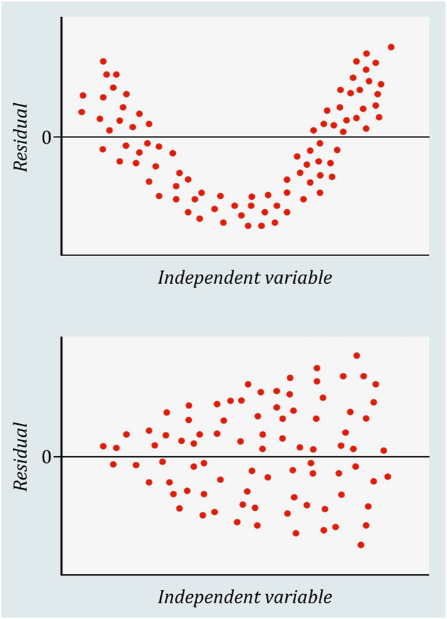
“So, the homework was to explain the key assumptions of the linear regression model by using the residual plot.” Mumbling, the student drew a couple of scatter plots with a horizontal line at the y of zero (Figure 1).

Note: The x-axis can be the predicted (fitted) values.
Figure 1 Examples of the residual plot when the assumptions of linear regression do not hold.

He continued, “These are examples of the residual plot. How do we draw the plots? It’s easy. Scatter the residuals on the y-axis over its corresponding values of the independent variable on the x-axis. The first plot on the board is U-shaped, and the second looks like an arrowhead. The point is, there are patterns—more specifically, non-random patterns. What does this mean? Let’s recall the assumptions. After controlling for the independent variable or covariates, the residuals should not be correlated with each other. In addition, the residuals at any value of the independent variable should be normally distributed, sharing the same variance. Simply put, the pattern should be…” The student erased the plots and drew another (Figure 2).

Figure 2 The residual plot from a linear model where the assumptions hold.

“…none. Or maybe we can call it a non-random pattern, meaning the linear model explains the patterns, if there are any. So there is no pattern left among the residuals, as it should be. The bottom line is, the residual plot is a litmus test that proves whether the assumptions of linear regression holds. If a random scatter pattern is observed, then the linear model is a decent choice; if not, a non-linear model should be applied. In the U-shaped plot, we can consider using a quadratic model.” The student explained the conclusion with confidence, speaking very fast, just like Sherlock.

“Seems like you got the point,” John said, but the student hurriedly spoke once again.

“Wait, wait. I have a question for Sherlock. I understand why you gave me the homework, but I have not seen residual plot testing the assumptions of regression in any articles I have read. When would I use it in reality?”

Sherlock chuckled. “Well, I think journals have an unbounded assumption that every researcher does his duty checking the soundness of the model before submitting a manuscript. Or, practically speaking, the usual 3,000-word limit is too short to deal with this litmus test. However, I strongly suggest you include this kind of information in your dissertation. There’s no word limit when writing a thesis, is there?”

“I see.” The student looked satisfied.

Sherlock added, “And, when you describe the equal variance, you may want to use the term, ‘homoscedasticity’. The antonym is, of course, ‘heteroscedasticity’. Except for the difficulty experienced when pronouncing them, they will serve as such a powerful weapon in an article or any presentation that they may overwhelm the audience.”

John thought, That’s typical of how Sherlock thinks.

Sherlock offered a final remark while pushing the student out of his flat. “So, you are ready for linear regression. Go back to your room and begin to re-write your dissertation. Next time, if we have time before your final defence, I will teach you how to apply a multilevel component to your model.”

“Thanks a lot,” the student said as firmly, still holding Sherlock’s hand.
John saw Sherlock smile at the student, and it was a smile to a colleague.